16.2. Improved approach

Corotational setting

StrainSmall

DisplacementLarge

MaterialLinear elastic

Stress statePlane stress

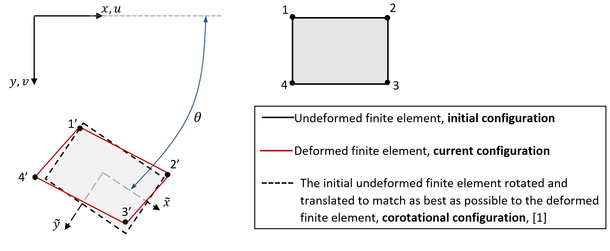
As in Section 16.1, the rigid-body motion is removed by replacing the initial configuration with the corotational configuration. The analysis is performed on the current deformed configuration [1, 2].

Initial, current, and corotational configurations of a Q4 element — **Figure 1.** Initial undeformed, current deformed, and corotational configurations of the 4-node quadrilateral finite element.

The nodal coordinates and displacements are:

\boldsymbol{x}=\begin{Bmatrix}x\\y\end{Bmatrix}\qquad \boldsymbol{u}=\begin{Bmatrix}u\\v\end{Bmatrix}

The configurations and corotational nodal displacements are:

\boldsymbol{x}_{el}=\boldsymbol{x}_{el0}+\boldsymbol{u}_{el}

\widetilde{\boldsymbol{x}}_{el}=\boldsymbol{R}\boldsymbol{x}_{el0}\qquad\text{with}\qquad\boldsymbol{R}=\begin{bmatrix}\cos\theta&\sin\theta\\-\sin\theta&\cos\theta\end{bmatrix}

\widetilde{\boldsymbol{u}}_{el}=\boldsymbol{x}_{el}-\widetilde{\boldsymbol{x}}_{el}=(\boldsymbol{I}_2-\boldsymbol{R})\boldsymbol{x}_{el0}+\boldsymbol{u}_{el}

The engineering strain measure is used for the small deformational part:

\left\{\begin{aligned}\varepsilon_x&=\frac{\partial u}{\partial x}\\[3pt]\varepsilon_y&=\frac{\partial v}{\partial y}\\[3pt]\gamma_{xy}&=\frac{\partial u}{\partial y}+\frac{\partial v}{\partial x}\end{aligned}\right.

\left\{\begin{aligned}\varepsilon_x&=\frac{\partial\widetilde{u}}{\partial x}\\[3pt]\varepsilon_y&=\frac{\partial\widetilde{v}}{\partial y}\\[3pt]\gamma_{xy}&=\frac{\partial\widetilde{u}}{\partial y}+\frac{\partial\widetilde{v}}{\partial x}\end{aligned}\right.

These relations are equivalent because $(\boldsymbol{I}_2-\boldsymbol{R})\boldsymbol{x}_0$ is constant within the element; see Section 16.1.

Equilibrium and improved tangent approximation

The nonlinear equilibrium equations are:

\boldsymbol{\Psi}(\boldsymbol{u})=\mathcal{A}_{el=1}^{n_{el}}\!\left(h\sum_{n_G}\boldsymbol{B}^{T}\boldsymbol{\sigma}\det(\boldsymbol{J})\right)-\boldsymbol{F}=\boldsymbol{0}

\boldsymbol{\Psi}(\boldsymbol{u})=\mathcal{A}_{el=1}^{n_{el}}\!\left(\boldsymbol{f}_{el}\right)-\boldsymbol{F}=\boldsymbol{0}

Here, $\mathcal{A}$ denotes the standard finite-element assembly operator, $\sum_{n_G}$ represents Gauss quadrature for one element, and $n_{el}$ is the number of finite elements. The element internal-force vector is:

\boldsymbol{f}_{el}=h\sum_{n_G}\boldsymbol{B}^{T}\boldsymbol{\sigma}\det(\boldsymbol{J})

The stiffness matrix is defined through the derivative:

\boldsymbol{k}_{el}=\frac{\partial\boldsymbol{f}_{el}}{\partial\widetilde{\boldsymbol{u}}_{el}}

Because both $\boldsymbol{B}$ and $\boldsymbol{J}$ depend on $\widetilde{\boldsymbol{u}}_{el}$ , the contributions retained in the improved tangent approximation are:

\boldsymbol{k}_{el}=\sum_{n_G}\!\left(\underbrace{h\det(\boldsymbol{J})\boldsymbol{B}^{T}\frac{\partial\boldsymbol{\sigma}}{\partial\widetilde{\boldsymbol{u}}_{el}}}_{T_1}+\underbrace{h\det(\boldsymbol{J})\frac{\partial\boldsymbol{B}^{T}}{\partial\widetilde{\boldsymbol{u}}_{el}}\boldsymbol{\sigma}}_{T_2}+\underbrace{h\frac{\partial|\det\boldsymbol{J}|}{\partial\widetilde{\boldsymbol{u}}_{el}}\boldsymbol{B}^{T}\boldsymbol{\sigma}}_{T_3}\right)

The internal nodal force vector $\boldsymbol{f}_{el}$ is evaluated consistently and is the quantity that governs the equilibrium solution. The stiffness matrix $\boldsymbol{k}_{el}$ used here is not the complete derivative of $\boldsymbol{f}_{el}$ , because not all dependencies introduced by the corotational transformation are differentiated. However, the additional terms included in this section provide a much better tangent approximation than in Section 16.1 and substantially improve the convergence rate. Since $\boldsymbol{f}_{el}$ itself is correct, the iterative process still converges to the correct equilibrium solution.

The tangent stiffness matrix obtained with the present approximation is generally non-symmetric. For Example 1, the measured mean relative asymmetry of the element tangent matrices was approximately $7.37\times10^{-2}$ . No artificial symmetrization is applied, since numerical tests showed that symmetrization significantly deteriorates the convergence rate.

Contribution T1

The first contribution to the improved tangent approximation is:

T_1=h\sum_{n_G}\det(\boldsymbol{J})\boldsymbol{B}^{T}\frac{\partial\boldsymbol{\sigma}}{\partial\widetilde{\boldsymbol{u}}_{el}}

For a linear elastic material:

\boldsymbol{\sigma}=\boldsymbol{D}\boldsymbol{\varepsilon}=\boldsymbol{D}\boldsymbol{B}\widetilde{\boldsymbol{u}}_{el}

Consequently:

\frac{\partial\boldsymbol{\sigma}}{\partial\widetilde{\boldsymbol{u}}_{el}}=\frac{\partial(\boldsymbol{D}\boldsymbol{B}\widetilde{\boldsymbol{u}}_{el})}{\partial\widetilde{\boldsymbol{u}}_{el}}=\boldsymbol{D}\boldsymbol{B}

The resulting contribution is:

T_1=h\sum_{n_G}\det(\boldsymbol{J})\boldsymbol{B}^{T}\boldsymbol{D}\boldsymbol{B}=\boldsymbol{k}_{el1}

Contribution T2

The second contribution is:

T_2=h\sum_{n_G}\det(\boldsymbol{J})\frac{\partial\boldsymbol{B}^{T}}{\partial\widetilde{\boldsymbol{u}}_{el}}\boldsymbol{\sigma}=\boldsymbol{k}_{el2}

The derivative of $\boldsymbol{B}^{T}$ with respect to the eight-component element displacement vector is a collection of eight $8\times3$ matrices. For each degree of freedom, multiplication by the $3\times1$ stress vector:

\boldsymbol{\sigma}=\begin{Bmatrix}\sigma_x\\\sigma_y\\\tau_{xy}\end{Bmatrix}

produces one $8\times1$ column of $\boldsymbol{k}_{el2}$ . The complete $8\times8$ matrix is most conveniently identified by using virtual displacements:

\begin{aligned}h\sum_{n_G}\det(\boldsymbol{J})\,\delta\boldsymbol{B}^{T}\boldsymbol{\sigma}=h\sum_{n_G}\det(\boldsymbol{J})\Biggl(&\frac{\partial\boldsymbol{B}^{T}}{\partial\widetilde{u}_1}\boldsymbol{\sigma}\,\delta\widetilde{u}_1+\frac{\partial\boldsymbol{B}^{T}}{\partial\widetilde{v}_1}\boldsymbol{\sigma}\,\delta\widetilde{v}_1\\&+\frac{\partial\boldsymbol{B}^{T}}{\partial\widetilde{u}_2}\boldsymbol{\sigma}\,\delta\widetilde{u}_2+\frac{\partial\boldsymbol{B}^{T}}{\partial\widetilde{v}_2}\boldsymbol{\sigma}\,\delta\widetilde{v}_2\\&+\frac{\partial\boldsymbol{B}^{T}}{\partial\widetilde{u}_3}\boldsymbol{\sigma}\,\delta\widetilde{u}_3+\frac{\partial\boldsymbol{B}^{T}}{\partial\widetilde{v}_3}\boldsymbol{\sigma}\,\delta\widetilde{v}_3\\&+\frac{\partial\boldsymbol{B}^{T}}{\partial\widetilde{u}_4}\boldsymbol{\sigma}\,\delta\widetilde{u}_4+\frac{\partial\boldsymbol{B}^{T}}{\partial\widetilde{v}_4}\boldsymbol{\sigma}\,\delta\widetilde{v}_4\Biggr)\\&=\boldsymbol{k}_{el2}\,\delta\widetilde{\boldsymbol{u}}_{el}\end{aligned}

For each nodal degree of freedom, the corresponding derivative contributes one column to the matrix $\boldsymbol{k}_{el2}$ . The derivative with respect to the first degree of freedom gives the first column, and the remaining derivatives give the subsequent columns. As in Section 9.4:

\boldsymbol{b}=\boldsymbol{J}^{-1}\boldsymbol{H}=\begin{bmatrix}b_{11}&b_{12}&b_{13}&b_{14}\\b_{21}&b_{22}&b_{23}&b_{24}\end{bmatrix}

where the $2\times4$ matrix $\boldsymbol{H}$ is:

\boldsymbol{H}(s,t)=\frac14\begin{bmatrix}1+t&-(1+t)&-(1-t)&1-t\\1+s&1-s&-(1-s)&-(1+s)\end{bmatrix}

The Jacobian is evaluated from the nodal coordinates of the current configuration:

\boldsymbol{J}(s,t)=\boldsymbol{H}(s,t)\begin{bmatrix}x_1&y_1\\x_2&y_2\\x_3&y_3\\x_4&y_4\end{bmatrix}

\boldsymbol{x}_{el}=\begin{bmatrix}x_1&x_2&x_3&x_4\end{bmatrix}^{T}\qquad\boldsymbol{y}_{el}=\begin{bmatrix}y_1&y_2&y_3&y_4\end{bmatrix}^{T}

The strain-displacement matrix obtained from $\boldsymbol{b}$ is:

\boldsymbol{B}(s,t)=\begin{bmatrix}b_{11}&0&b_{12}&0&b_{13}&0&b_{14}&0\\0&b_{21}&0&b_{22}&0&b_{23}&0&b_{24}\\b_{21}&b_{11}&b_{22}&b_{12}&b_{23}&b_{13}&b_{24}&b_{14}\end{bmatrix}

The matrix $\boldsymbol{H}$ does not depend on the current nodal coordinates. The variation of $\boldsymbol{b}$ is obtained successively from:

\boldsymbol{b}=\boldsymbol{J}^{-1}\boldsymbol{H}\quad\Longrightarrow\quad\boldsymbol{J}\boldsymbol{b}=\boldsymbol{H}\quad\Longrightarrow\quad\delta\boldsymbol{J}\boldsymbol{b}+\boldsymbol{J}\delta\boldsymbol{b}=\boldsymbol{0}\quad\Longrightarrow\quad\delta\boldsymbol{b}=-\boldsymbol{J}^{-1}\delta\boldsymbol{J}\boldsymbol{b}

The eight element displacement variations enter the Jacobian through:

\begin{aligned}\delta\boldsymbol{J}=\boldsymbol{H}\Biggl(&\begin{bmatrix}1&0\\0&0\\0&0\\0&0\end{bmatrix}\delta\widetilde{u}_1+\begin{bmatrix}0&1\\0&0\\0&0\\0&0\end{bmatrix}\delta\widetilde{v}_1+\begin{bmatrix}0&0\\1&0\\0&0\\0&0\end{bmatrix}\delta\widetilde{u}_2+\begin{bmatrix}0&0\\0&1\\0&0\\0&0\end{bmatrix}\delta\widetilde{v}_2\\&+\begin{bmatrix}0&0\\0&0\\1&0\\0&0\end{bmatrix}\delta\widetilde{u}_3+\begin{bmatrix}0&0\\0&0\\0&1\\0&0\end{bmatrix}\delta\widetilde{v}_3+\begin{bmatrix}0&0\\0&0\\0&0\\1&0\end{bmatrix}\delta\widetilde{u}_4+\begin{bmatrix}0&0\\0&0\\0&0\\0&1\end{bmatrix}\delta\widetilde{v}_4\Biggr)\end{aligned}

Thus, $\partial\boldsymbol{J}/\partial\widetilde{\boldsymbol{u}}_{el}$ contains eight $2\times2$ matrices. The sequence of derivative dimensions is:

\frac{\partial\boldsymbol{J}}{\partial\widetilde{\boldsymbol{u}}_{el}}:\ 8\text{ matrices of size }2\times2

\frac{\partial\boldsymbol{b}}{\partial\widetilde{\boldsymbol{u}}_{el}}:\ 8\text{ matrices of size }2\times4

\frac{\partial\boldsymbol{B}}{\partial\widetilde{\boldsymbol{u}}_{el}}:\ 8\text{ matrices of size }3\times8

\frac{\partial\boldsymbol{B}^{T}}{\partial\widetilde{\boldsymbol{u}}_{el}}:\ 8\text{ matrices of size }8\times3

Multiplying each last matrix by $\boldsymbol{\sigma}$ produces an $8\times1$ column; the eight columns form the $8\times8$ contribution $\boldsymbol{k}_{el2}$ . The MATLAB implementation performs these operations directly:

% B derivative contribution:
for i=1:8
    p=zeros(2,4);
    p(i)=1;
    dJ=H*p';
    % derivative of b with respect to u_el:
    db=-J1*dJ*b;
    dBi=[db(1,1)       0    db(1,2)       0    db(1,3)       0    db(1,4)       0
            0    db(2,1)       0    db(2,2)       0    db(2,3)       0    db(2,4)
         db(2,1) db(1,1) db(2,2) db(1,2) db(2,3) db(1,3) db(2,4) db(1,4)];
    dBsig(:,i)=dBi'*sg;
end

Thus, the contribution is added as dBsig:

kel=kel+th1*(B'*DHooke*B+dBsig)*detJ + th1*ddetJ;

Contribution T3

The third contribution is:

T_3=h\sum_{n_G}\frac{\partial|\det\boldsymbol{J}|}{\partial\widetilde{\boldsymbol{u}}_{el}}\boldsymbol{B}^{T}\boldsymbol{\sigma}=\boldsymbol{k}_{el3}

Writing the determinant derivative component by component gives:

\frac{\partial\det(\boldsymbol{J})}{\partial\widetilde{\boldsymbol{u}}_{el}}=\begin{bmatrix}\dfrac{\partial\det(\boldsymbol{J})}{\partial\widetilde{u}_1}&\dfrac{\partial\det(\boldsymbol{J})}{\partial\widetilde{v}_1}&\dfrac{\partial\det(\boldsymbol{J})}{\partial\widetilde{u}_2}&\dfrac{\partial\det(\boldsymbol{J})}{\partial\widetilde{v}_2}&\dfrac{\partial\det(\boldsymbol{J})}{\partial\widetilde{u}_3}&\dfrac{\partial\det(\boldsymbol{J})}{\partial\widetilde{v}_3}&\dfrac{\partial\det(\boldsymbol{J})}{\partial\widetilde{u}_4}&\dfrac{\partial\det(\boldsymbol{J})}{\partial\widetilde{v}_4}\end{bmatrix}^{T}

Because the numerical integration uses $|\det\boldsymbol{J}|$ , its derivative must retain the sign of the signed determinant:

\frac{\partial|\det\boldsymbol{J}|}{\partial\widetilde{\boldsymbol{u}}_{el}}=\operatorname{sign}(\det\boldsymbol{J})\frac{\partial\det\boldsymbol{J}}{\partial\widetilde{\boldsymbol{u}}_{el}}

For the Q4 element:

\frac{\partial\det(\boldsymbol{J})}{\partial\widetilde{\boldsymbol{u}}_{el}}=\frac{1}{8}\begin{Bmatrix}y_2-y_4+s(y_3-y_4)+t(y_2-y_3)\\x_4-x_2-s(x_3-x_4)-t(x_2-x_3)\\y_3-y_1-s(y_3-y_4)-t(y_1-y_4)\\x_1-x_3+s(x_3-x_4)+t(x_1-x_4)\\y_4-y_2-s(y_1-y_2)+t(y_1-y_4)\\x_2-x_4+s(x_1-x_2)-t(x_1-x_4)\\y_1-y_3+s(y_1-y_2)-t(y_2-y_3)\\x_3-x_1-s(x_1-x_2)+t(x_2-x_3)\end{Bmatrix}

Here, $s$ and $t$ are the natural coordinates introduced for the Q4 element in Section 9.4. The implementation is:

detJs=det(J);
detJ=abs(detJs);
sgnJ=sign(detJs);

% Contribution of abs(det(J)):
x1=xdel(1); x2=xdel(2); x3=xdel(3); x4=xdel(4);
y1=ydel(1); y2=ydel(2); y3=ydel(3); y4=ydel(4);
ddJ=[y2-y4+s*y3-s*y4+t*y2-t*y3
     x4-x2-s*x3+s*x4-t*x2+t*x3
     y3-y1-s*y3+s*y4-t*y1+t*y4
     x1-x3+s*x3-s*x4+t*x1-t*x4
     y4-y2-s*y1+s*y2+t*y1-t*y4
     x2-x4+s*x1-s*x2-t*x1+t*x4
     y1-y3+s*y1-s*y2-t*y2+t*y3
     x3-x1-s*x1+s*x2+t*x2-t*x3];
ddetJ=sgnJ*ddJ*(B'*sg)'/8;

MATLAB implementation

The three retained tangent contributions are assembled in stiff.m as:

strn=B*sel;
strnt(ig,:,istep)=strn';
sg=DHooke*strn;
sigmt(ig,1:3,istep)=sg';
sgr=R'*[sg(1), sg(3); sg(3), sg(2)]*R;
sigmtr(ig,1:3,istep)=[sgr(1,1), sgr(2,2), sgr(1,2)];
deltaB

th1=(1-nu/(1-nu)*(strn(1)+strn(2)))*th;
fel=fel+th1*(B'*sg)*detJ;
kel=kel+th1*(B'*DHooke*B+dBsig)*detJ + th1*ddetJ;

The Cauchy stress in the element local frame is obtained from:

\widetilde{\boldsymbol{\sigma}}=\boldsymbol{R}^{T}\boldsymbol{\sigma}\boldsymbol{R}

The stresses are evaluated both in the global and in the local reference frame. This is very easy to do, because the rotation matrix $\boldsymbol{R}$ has already been computed for determining the corotational configuration; therefore, no additional computational effort is required.

For side $i$ , let $\boldsymbol{d}_i^0$ be its vector in the initial configuration and $\boldsymbol{d}_i^c$ the homologous vector in the current configuration. The signed rotation is:

\theta_i=\operatorname{atan2}\left((\boldsymbol{d}_i^c\times\boldsymbol{d}_i^0)_z,\,\boldsymbol{d}_i^c\cdot\boldsymbol{d}_i^0\right)

The representative element rotation remains the arithmetic average:

\theta=\frac14\left(\theta_{12}+\theta_{23}+\theta_{34}+\theta_{41}\right)

The corresponding MATLAB sequence is:

cr=cross(dxyd,dxy);
dt=dot(dxyd,dxy);
thet(i)=atan2(cr(3),dt);

thetm=mean(thet);

The current thickness is updated using the same small-strain plane-stress approximation:

\varepsilon_z=-\frac{\nu}{1-\nu}(\varepsilon_x+\varepsilon_y)\qquad h_{\mathrm{cur}}\approx(1+\varepsilon_z)h

This thickness relation is a small-strain approximation; it is not a general exact relation for finite elastic strains.

Examples

Example 1 — pure bending

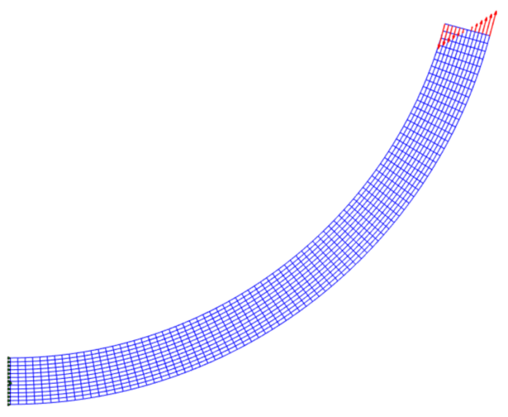
A cantilever beam has $L=400\,\mathrm{mm}$ , rectangular cross-section $5\,\mathrm{mm}\times30\,\mathrm{mm}$ , $E=1000\,\mathrm{MPa}$ , and $\nu=0.3$ . A bending moment $M=37000\,\mathrm{N\,mm}$ is applied through forces at the free end. The structured mesh contains $80\times12=960$ Q4 elements and 1053 nodes. This is the default problem generated by gen1.m.

The theoretical bending angle is:

\varphi=\frac{CL}{EI}=\frac{37000\cdot400}{1000(30^3\cdot5/12)}=1.31\,\mathrm{rad}=75^\circ

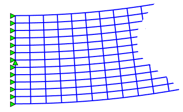
Intermediate deformed configurations of Example 1 — **Figure 2.** Intermediate deformed configurations during loading.

Final deformed configuration of Example 1 — **Figure 3.** Final deformed configuration for the pure-bending example.

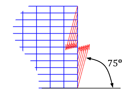
The forces have a fixed orientation in space, as shown in Figure 4.

The forces increase proportionally with the load-step number, while their moment arms change as the beam deforms. Consequently, the resulting bending moment does not increase exactly proportionally with the load-step number.

Direction of the end forces at 75 degrees — **Figure 4.** End forces acting at $75^\circ$ to the horizontal.

End forces on the initial undeformed configuration — **Figure 5.** Forces shown on the initial undeformed configuration.

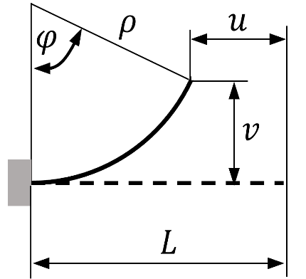
Elementary pure-bending geometry — **Figure 6.** Geometry used for the elementary displacement comparison.

Axial Cauchy stress in the local element frames for Example 1 — **Figure 7.** Axial Cauchy stress $\sigma_x$ in the local reference frames of the finite elements.

The classic bending formula gives:

\sigma_{\max}=\frac{C}{W}=\frac{6\cdot37000}{5\cdot30^2}=49.3\,\mathrm{MPa}

The MATLAB result ranges approximately from $-50.71\,\mathrm{MPa}$ to $50.52\,\mathrm{MPa}$ . The accompanying ANSYS comparison gives approximately $\sigma_{\min}=-49.91\,\mathrm{MPa}$ and $\sigma_{\max}=49.04\,\mathrm{MPa}$ .

The maximum axial strain is about 0.05. This is already a relatively large value for a small-strain formulation, but it is useful here because it makes the differences between the compared approaches more visible.

The midpoint displacements of the free end are compared below:

Formulation	$u$	$v$
TL	$-105.04\,\mathrm{mm}$	$227.11\,\mathrm{mm}$
UL	$-103.00\,\mathrm{mm}$	$226.08\,\mathrm{mm}$
CR	$-104.54\,\mathrm{mm}$	$227.02\,\mathrm{mm}$
ANSYS	$-104.50\,\mathrm{mm}$	$226.81\,\mathrm{mm}$

The elementary circular-arc estimate uses:

\rho=\frac{L}{\varphi}=\frac{400}{1.31}=305.34\,\mathrm{mm}

u=L-\rho\sin\varphi=400-305.34\sin(1.31)=104.98\,\mathrm{mm}

v=\rho(1-\cos\varphi)=305.34\bigl(1-\cos(1.31)\bigr)=226.61\,\mathrm{mm}

Example 2 — cantilever loaded by an end force

The beam has $L=400\,\mathrm{mm}$ , rectangular cross-section $5\,\mathrm{mm}\times20\,\mathrm{mm}$ , $E=1000\,\mathrm{MPa}$ , $\nu=0.3$ , and an end force $F=100\,\mathrm{N}$ . The mesh contains $60\times8=480$ Q4 elements, 549 nodes, and 8 load steps. Run this problem by replacing gen1 with gen2 in main.m.

Axial Cauchy stress for Example 2 — **Figure 8.** Axial Cauchy stress $\sigma_x$ for Example 2 at load step 8.

Convergence and load stepping

The additional tangent contributions substantially accelerate convergence compared with Section 16.1. For $\mathrm{tol}=10^{-5}$ , the examples considered required approximately 8–9 iterations per load step with $n_{\mathrm{step}}=5$ , and typically 6–8 iterations per load step with $n_{\mathrm{step}}=10$ . These are results for the present examples, not universal convergence guarantees.

Important remark. The corotational formulation presented here is not incremental with respect to the strain or reference configuration. The converged final solution does not depend on the number of load steps. Load stepping may nevertheless be used to facilitate convergence or to follow the response of the structure during loading, for example to obtain a force–displacement curve. If only the final state is required and convergence is achieved, a single load step gives the same final result.

Program and download

The MATLAB package used for the two examples can be downloaded below.

MMATLAB packageDOWNLOAD ZIP

References

Lagrangian and Corotational Formulations, Altair, 2021.
Felippa, C. A., Nonlinear Finite Element Methods, Department of Aerospace Engineering Sciences, University of Colorado at Boulder, Chapters 12 and 13, 2004.