Nomenclature and Conventions

Notation

Scalars are written with italic letters. Vectors and matrices are written with bold italic letters.

Abstract vector and matrix symbols are written without brackets. When their components are displayed explicitly, a row vector uses parentheses, a column vector uses braces, and a matrix uses square brackets.

$\Pi,\ U,\ V,\ E,\ A,\ L,\ u$: Scalars
$\boldsymbol{K},\ \boldsymbol{k}_{el},\ \boldsymbol{f}_{el},\ \boldsymbol{u},\ \boldsymbol{u}_{el}$: Vectors and matrices. Their dimensions follow from context: for example, $\boldsymbol{u}$ and $\boldsymbol{f}_{el}$ are column vectors, whereas $\boldsymbol{K}$ and $\boldsymbol{k}_{el}$ are matrices.
$\overline{\boldsymbol{K}},\ \overline{\boldsymbol{k}}_{el},\ \overline{\boldsymbol{f}}_{el},\ \overline{\boldsymbol{u}}$: A bar denotes a vector or tensor expressed in the local reference frame. Symbols without a bar refer to the global reference frame.

Symbols

Latin symbols

$A_{el},\ A$: Finite-element area; cross-sectional area
$A_0$: Effective shear area
$\mathcal{A}$: Finite-element assembly operator; see Assembly paragraph
$\boldsymbol{B}$: Strain-displacement matrix
$\boldsymbol{B}_0$: Linear part of the strain-displacement matrix
$\boldsymbol{B}_L$: Nonlinear part of the strain-displacement matrix
$\boldsymbol{b}=\boldsymbol{F}\boldsymbol{F}^{T}$: Left Cauchy–Green tensor
$\boldsymbol{C}$: Quadratic strain matrix used to form the truss geometric stiffness matrix
$\boldsymbol{D}$: Constitutive matrix, with $\boldsymbol{\sigma}=\boldsymbol{D}\boldsymbol{\varepsilon}$
$E$: Young's modulus
$E_t=\dfrac{d\sigma}{d\varepsilon}$: Tangent modulus
$\boldsymbol{E}$: Green–Lagrange strain tensor
$\boldsymbol{E}_{\mathrm{GL}}$: Green–Lagrange strain measure
$\boldsymbol{e}$: Euler–Almansi strain tensor
$\boldsymbol{e}_{\mathrm{EA}}$: Euler–Almansi strain measure
$\boldsymbol{F}$: Nodal-force vector
$\boldsymbol{F}$: Deformation gradient
$\boldsymbol{F}_{\Delta}$: Incremental deformation gradient
$\boldsymbol{F}_{\mathrm{tot}}$: Total deformation gradient
$F,\ V,\ H$: Force components
$\begin{gathered}F(\psi,m),\ K(m)\\E(\psi,m),\ E(m)\end{gathered}$: $F(\psi,m)$ and $K(m)$ are the incomplete and complete elliptic integrals of the first kind; $E(\psi,m)$ and $E(m)$ are the corresponding integrals of the second kind. Here $F(\cdot)$ and $E(\cdot)$ denote elliptic-integral functions, not force and Young's modulus
$G$: Shear modulus
$\boldsymbol{G}_x,\ \boldsymbol{G}_y,\ \boldsymbol{G}_{xy},\ldots$: Symmetric matrices associated with the nonlinear part of the Green-Lagrange strains
$\boldsymbol{H}$: Matrix used to calculate the Jacobian matrix, $\boldsymbol{J}=\boldsymbol{H}[\boldsymbol{x}_{el}\ \boldsymbol{y}_{el}\ \boldsymbol{z}_{el}]$
$I$: Second moment of area, generic
$I_1,\ I_2$: Principal second moments of area
$I_y$: Second moment of area about the $y$ -axis
$I_z$: Second moment of area about the $z$ -axis
$I_t$: Cross-sectional torsion constant
$\boldsymbol{I}_{r}$: Identity matrix of order $r$ , with $r=2$ for a plane truss and $r=3$ for a spatial truss
$\boldsymbol{J}$: Jacobian matrix
$\boldsymbol{K},\ \boldsymbol{k},\ \boldsymbol{k}_{el}$: Elastic or tangent stiffness matrices, as specified in context
$\boldsymbol{a}$: Compact vector of deformed element coordinate differences used in exact truss strain derivatives
$\boldsymbol{d}$: Unit vector along the initial axis of a truss element
$d\boldsymbol{a}$: Oriented differential area vector in the reference configuration
$d\hat{\boldsymbol{a}}$: Oriented differential area vector in the current configuration
$d\boldsymbol{f}$: Differential physical force vector
$dV_0$: Differential volume in the initial or reference configuration
$dV$: Differential volume in the current configuration
$\boldsymbol{G}$: Constant block matrix used in the exact Hessian of truss engineering strain
$\boldsymbol{K}_{G},\ \boldsymbol{k}_{G,el}$: Structural and element geometric stiffness matrices
$L,\ L_b$: Element length; beam length
$L_f$: Element length in the deformed configuration
$M$: Bending moment
$M_t$: Twisting moment or torque
$N$: Axial force
$\boldsymbol{N}$: Shape-function or interpolation-function matrix
$n_{el}$: Number of finite elements
$n_G,\ \xi_G,\ (s_G,t_G),\ w_G$: Number of Gauss points, Gauss-point coordinates, and Gauss weights
$\boldsymbol{P}=\boldsymbol{I}-\boldsymbol{d}\boldsymbol{d}^{T}$: Projector onto directions transverse to a truss element axis
$\boldsymbol{P}$: First Piola–Kirchhoff stress tensor
$\boldsymbol{p}=\begin{pmatrix}-\boldsymbol{d}^{T}&\boldsymbol{d}^{T}\end{pmatrix}^{T}$: Element nodal vector constructed from the initial truss-axis unit vector
$\boldsymbol{Q}_{r}$: Dimension-independent block matrix $\begin{bmatrix}\boldsymbol{I}_{r}&-\boldsymbol{I}_{r}\\-\boldsymbol{I}_{r}&\boldsymbol{I}_{r}\end{bmatrix}$ for a truss in $r$ dimensions
$\boldsymbol{R}$: Rotation matrix
$\boldsymbol{S}$: Second Piola–Kirchhoff stress tensor
$T$: Shear force
$U$: Strain energy
$V$: Potential of the applied loads
$\boldsymbol{f}_{el}$: Internal nodal-force vector for one finite element
$h$: Thickness
$h_1,\ h_2$: Shape functions
$l,\ m,\ n$: Direction cosines
$k,\ m=k^2$: Elliptic modulus and elliptic parameter in the cantilever elastica solution
$r$: Radial coordinate
$s$: Curvilinear coordinate
$s,\ t,\ r$: Natural coordinates for isoparametric finite elements
$u,\ v,\ w$: Displacement components
$\boldsymbol{u},\ \boldsymbol{u}_{el}$: Structural and element nodal-displacement vectors
$\nabla\boldsymbol{u}$: Displacement gradient
$\widetilde{\boldsymbol{u}}$: Corotated nodal-displacement vector
$\mathcal{V},\ \mathcal{V}_{el}$: Volume; finite-element volume
$x,\ y,\ z$: Cartesian coordinates
$\hat{\boldsymbol{x}}$: Position vector in the current or deformed configuration
$\widetilde{\boldsymbol{x}}$: Coordinates or position vector in the corotational configuration

Greek symbols

$\beta$: Shear angle, or the fixed force-direction angle in the cantilever elastica solution, as specified in context
$\gamma$: Dimensionless correction factor for the one-point shear contribution in the isoparametric Timoshenko beam element
$\delta$: Prefix denoting a virtual quantity
$\Delta=\det\boldsymbol{F}$: Local volume ratio or determinant of the deformation gradient; this scalar quantity is distinct from $\Delta$ used as an increment symbol
$\Delta\boldsymbol{E}$: Green–Lagrange strain increment
$\Delta\boldsymbol{e}$: Euler–Almansi strain increment
$\epsilon$: Numerical error
$\varepsilon_0$: Beam axial strain
$\varepsilon_V$: Volumetric strain
$\varepsilon_x,\ \varepsilon_y,\ \gamma_{xy},\ldots$: Strain components
$\boldsymbol{\varepsilon}$: Strain vector or tensor
$\boldsymbol{\eta}=\frac{1}{L}\Delta\boldsymbol{u}$: Relative nodal-displacement vector normalized by the initial truss length
$\theta$: Polar angle or tangent-direction angle
$\kappa$: Curvature
$\boldsymbol{\kappa}$: Curvature vector or tensor
$\lambda$: Eigenvalue or buckling load factor
$\nu$: Poisson's ratio
$\xi$: Dimensionless coordinate, $\xi=x/L$
$\Pi$: Total potential energy
$\sigma_x,\ \sigma_y,\ \tau_{xy},\ldots$: Stress components
$\sigma_{\mathrm{VM}}$: Von Mises equivalent stress
$\boldsymbol{\sigma}$: Stress vector or tensor
$\widetilde{\boldsymbol{\sigma}}$: Stress tensor or components referred to the corotational or local frame
$\varphi$: Rotation of the normal
$\boldsymbol{\varphi}$: Rotation vector
$\boldsymbol{\phi}$: Buckling eigenvector or mode shape
$\psi$: Cross-section rotation
$\boldsymbol{\Psi}=\partial\Pi/\partial\boldsymbol{u}$: Equilibrium residual; the equilibrium equations are $\boldsymbol{\Psi}=\boldsymbol{0}$

Derivative notation

$\begin{gathered}u_{,x}\equiv\dfrac{\partial u}{\partial x}\\[3pt]u_{,xy}\equiv\dfrac{\partial^2u}{\partial x\,\partial y}\end{gathered}$: A comma in the subscript denotes differentiation with respect to the coordinate that follows it. For example, the expressions shown give first- and mixed second-derivative forms.

Variable names in MATLAB programs

The following list contains the principal names used in the accompanying programs.

A, Ael: Finite-element area; cross-sectional area
B, B0, BL: Strain-displacement matrices
cond: Table of nodal constraints
D, DHooke: Constitutive matrices
E: Young's modulus
elem: Finite-element connectivity and properties
ep, ep1, ep2: Engineering strain, strain gradient, and strain Hessian in the truss programs
ep, ca, be: Beam axial strain, curvature, and shear angle
F: Nodal-force vector
fel: Element internal-force vector
forze: Table of externally applied nodal loads
G: Shear modulus
ip: Element degree-of-freedom locations
istep, nstep: Current and total number of load steps
K, kel, KG, kelG: Structural elastic, element elastic, structural geometric, and element geometric stiffness matrices
lambda, Vfree: Buckling load factors and free-degree-of-freedom eigenvectors
L, l: Element or beam length
m, k, psi, psi0, thetaA: Elliptic parameter, elliptic modulus, transformed angles, and free-end tangent angle in the cantilever program
nel: Number of finite elements
neq: Number of structural degrees of freedom
nnd: Number of nodes
nu: Poisson's ratio
S: Structural nodal-displacement vector; the name comes from the Italian spostamenti
u, v, w: Nodal displacement components
uel: Element nodal-displacement vector
ux, uy, vz, wx, ...: Derivatives of displacement components
xy, xyz, x, y, z: Cartesian nodal coordinates

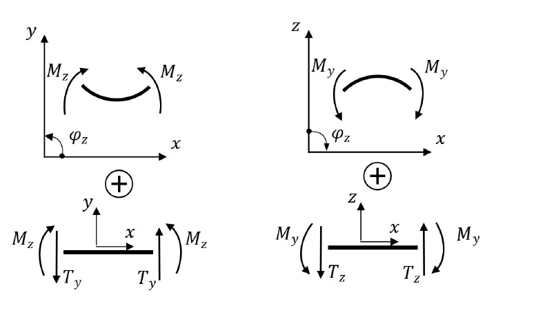
Sign convention for beams

Axial force and normal stress are positive in tension and negative in compression.

Chapter 4 retains the coordinate convention used in its finite-difference derivation: the global $x$ axis points to the right and its $y$ axis points downward. This chapter-specific choice is stated in its figure and MATLAB program.

In planar analyses, $T$ and $T_y$ denote the same transverse force component, while $M$ and $M_z$ denote the same bending moment component.

Bending

\varphi_z=\frac{dv}{dx}

\varphi_y=-\frac{dw}{dx}

\kappa_z=\frac{d\varphi_z}{dx}=\frac{d^2v}{dx^2}

\kappa_y=\frac{d\varphi_y}{dx}=-\frac{d^2w}{dx^2}

\frac{dM_z}{dx}=-T_y

\frac{dM_y}{dx}=T_z

\frac{d^2v}{dx^2}=\frac{M_z}{EI_z}

\frac{d^2w}{dx^2}=-\frac{M_y}{EI_y}

Matrix calculus conventions

Partial derivatives

For a two-dimensional truss element with four degrees of freedom,

\boldsymbol{u}_{el}=\begin{pmatrix}u_1&v_1&u_2&v_2\end{pmatrix}^{T}

\frac{\partial}{\partial\boldsymbol{u}_{el}}=\begin{Bmatrix}\dfrac{\partial}{\partial u_1}\\[3pt]\dfrac{\partial}{\partial v_1}\\[3pt]\dfrac{\partial}{\partial u_2}\\[3pt]\dfrac{\partial}{\partial v_2}\end{Bmatrix}

\frac{\partial^2}{\partial\boldsymbol{u}_{el}^2}=\begin{bmatrix}\dfrac{\partial^2}{\partial u_1^2}&\dfrac{\partial^2}{\partial u_1\partial v_1}&\dfrac{\partial^2}{\partial u_1\partial u_2}&\dfrac{\partial^2}{\partial u_1\partial v_2}\\[3pt]\dfrac{\partial^2}{\partial v_1\partial u_1}&\dfrac{\partial^2}{\partial v_1^2}&\dfrac{\partial^2}{\partial v_1\partial u_2}&\dfrac{\partial^2}{\partial v_1\partial v_2}\\[3pt]\dfrac{\partial^2}{\partial u_2\partial u_1}&\dfrac{\partial^2}{\partial u_2\partial v_1}&\dfrac{\partial^2}{\partial u_2^2}&\dfrac{\partial^2}{\partial u_2\partial v_2}\\[3pt]\dfrac{\partial^2}{\partial v_2\partial u_1}&\dfrac{\partial^2}{\partial v_2\partial v_1}&\dfrac{\partial^2}{\partial v_2\partial u_2}&\dfrac{\partial^2}{\partial v_2^2}\end{bmatrix}

Useful derivatives

For constant vectors $\boldsymbol{F}$ and a constant matrix $\boldsymbol{K}$ ,

\frac{\partial(\boldsymbol{u}^{T}\boldsymbol{F})}{\partial\boldsymbol{u}}=\boldsymbol{F}

\frac{\partial(\boldsymbol{u}^{T}\boldsymbol{K}\boldsymbol{u})}{\partial\boldsymbol{u}}=(\boldsymbol{K}+\boldsymbol{K}^{T})\boldsymbol{u}

\frac{\partial^2(\boldsymbol{u}^{T}\boldsymbol{K}\boldsymbol{u})}{\partial\boldsymbol{u}^2}=\boldsymbol{K}+\boldsymbol{K}^{T}

If $\boldsymbol{K}$ is symmetric, these last two expressions reduce to $2\boldsymbol{K}\boldsymbol{u}$ and $2\boldsymbol{K}$ .

Assembly

With the usual finite-element placement of element quantities into their global degree-of-freedom positions,

\sum_{el}\boldsymbol{u}_{el}^{T}\boldsymbol{k}_{el}\boldsymbol{u}_{el}=\boldsymbol{u}^{T}\boldsymbol{K}\boldsymbol{u}

\sum_{el}\boldsymbol{k}_{el}\boldsymbol{u}_{el}=\boldsymbol{K}\boldsymbol{u},\qquad \sum_{el}\boldsymbol{k}_{el}=\boldsymbol{K}

On this site, the compact finite-element assembly notation:

\mathop{\mathcal{A}}_{el=1}^{n_{el}}

is preferred. It denotes the usual placement of element quantities into their corresponding global degree-of-freedom positions followed by summation over all finite elements. For example:

\boldsymbol{K}=\mathop{\mathcal{A}}_{el=1}^{n_{el}}\left(\boldsymbol{k}_{el}\right)

\boldsymbol{F}_{\mathrm{int}}=\mathop{\mathcal{A}}_{el=1}^{n_{el}}\left(\boldsymbol{f}_{el}\right)

Special quadratic form

For column vectors $\boldsymbol{u},\boldsymbol{a},\boldsymbol{b}\in\mathbb{R}^{n}$ ,

\Pi=\boldsymbol{u}^{T}(\boldsymbol{a}\boldsymbol{b}^{T})\boldsymbol{u}=\frac{1}{2}\boldsymbol{u}^{T}(\boldsymbol{a}\boldsymbol{b}^{T}+\boldsymbol{b}\boldsymbol{a}^{T})\boldsymbol{u}

The Hessian is the symmetric matrix

\frac{\partial^2\Pi}{\partial\boldsymbol{u}^2}=\boldsymbol{a}\boldsymbol{b}^{T}+\boldsymbol{b}\boldsymbol{a}^{T}

Virtual work and energy principles

For a linear elastic structure with a symmetric stiffness matrix, the total potential energy is

\Pi=\frac{1}{2}\sum_{el}\boldsymbol{u}_{el}^{T}\boldsymbol{k}_{el}\boldsymbol{u}_{el}-\boldsymbol{u}^{T}\boldsymbol{F}=\frac{1}{2}\boldsymbol{u}^{T}\boldsymbol{K}\boldsymbol{u}-\boldsymbol{u}^{T}\boldsymbol{F}

Minimum total potential energy

\boldsymbol{\Psi}=\frac{\partial\Pi}{\partial\boldsymbol{u}}=\boldsymbol{K}\boldsymbol{u}-\boldsymbol{F}=\boldsymbol{0}

Principle of virtual work

For every geometrically admissible virtual displacement $\delta\boldsymbol{u}$ ,

\delta\Pi=\delta\boldsymbol{u}^{T}\left(\boldsymbol{K}\boldsymbol{u}-\boldsymbol{F}\right)=0

Both principles lead to the same equilibrium equations:

\boldsymbol{K}\boldsymbol{u}=\boldsymbol{F}

Validation of Programs and Macros

The present website is a revised edition of material developed and validated over many years. Programs and macros transferred to this edition without technical modification are not necessarily re-executed during the current revision. When a program is modified, it is tested again whenever practical. MATLAB programs are actively maintained and may therefore be revalidated more frequently.