16.4. Short comparison of TL, UL and CR formulations

TL, UL, and CR formulations

CR is non-incremental like TL, but, like UL, it evaluates the element response in the current configuration and provides Cauchy stresses.

The main conceptual features of the three formulations are summarized below.

Feature	TL	UL	CR
Reference configuration	Initial and fixed	Updated configuration; the last accepted configuration is used as reference	Non-incremental: strains from the current corotated state; initial configuration used for rigid-body motion.
Character	Non-incremental	Incremental	Non-incremental; load steps may still facilitate convergence and trace the response
Strain measure	Green–Lagrange (GL)	Euler–Almansi (EA)	Engineering (eng)
Stress measure	Second Piola–Kirchhoff stress	Cauchy stress	Cauchy stress
Large rigid-body rotations	Rigid-body motion filtered intrinsically by GL strain	Rigid-body motion filtered intrinsically by EA strain	Rigid-body motion explicitly removed before engineering-strain evaluation
Response evaluated in	Initial reference configuration	Current configuration	Current/corotated configuration

For small deformational strains:

\boldsymbol{E}_{\mathrm{GL}}\approx\boldsymbol{e}_{\mathrm{EA}}\approx\boldsymbol{\varepsilon}_{\mathrm{eng}}

This approximation alone does not explain the close agreement between CR and UL. Their closer conceptual relation is that both evaluate the response using the current deformed geometry and both provide Cauchy stresses. After the rigid-body rotation has been removed in CR, the remaining engineering strains are close to Euler–Almansi strains when the deformational strains are small.

The strain measure itself does not impose a restriction on the load-step size. Green–Lagrange and Euler–Almansi strains are objective measures, so a pure rigid-body motion does not generate strain, regardless of whether the final rotation is reached in one load step or in several. The load-step size is instead related to the nonlinear solution procedure, path following, and any approximations introduced by the numerical implementation.

Numerical example

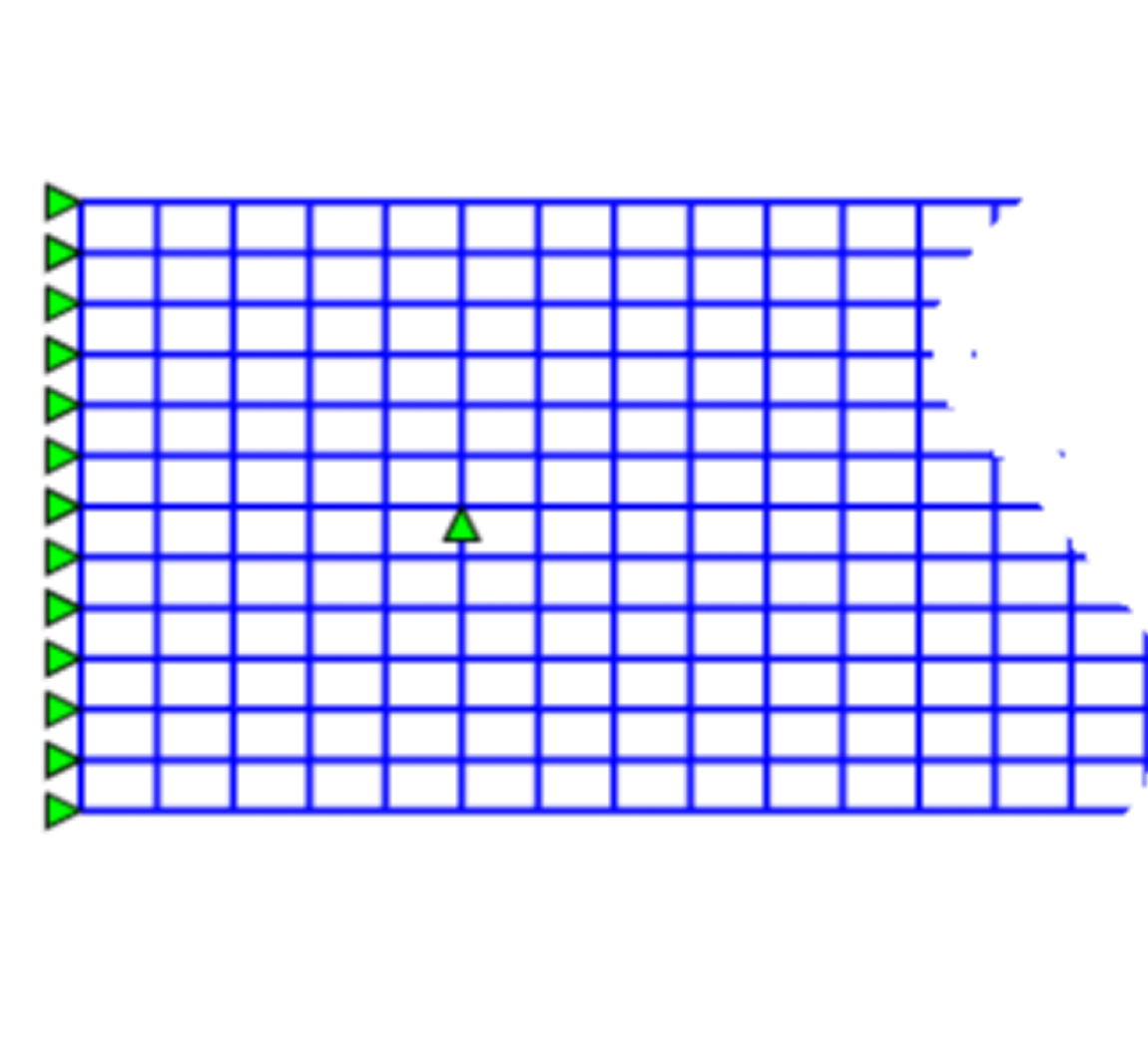
The cantilever has length $L=400\,\mathrm{mm}$ , rectangular cross-section $5\times40\,\mathrm{mm}$ , Young’s modulus $E=1000\,\mathrm{MPa}$ , and Poisson’s ratio $\nu=0.3$ . A force $F=800\,\mathrm{N}$ is applied. The mesh contains $80\times12=960$ 4-node isoparametric elements and $1053$ nodes.

To obtain an almost pure-bending state in the section of interest, only the horizontal displacements are constrained at the left end. A single vertical support is placed sufficiently far from this section so that it does not disturb the stress state there.

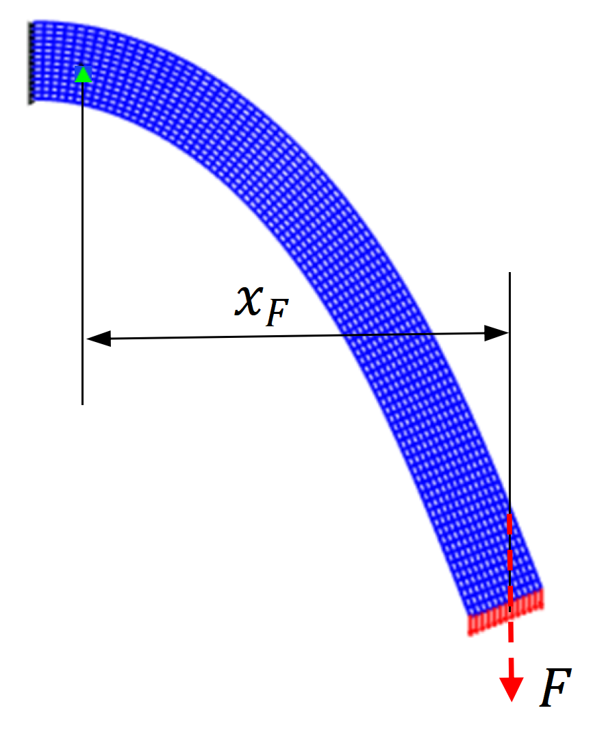
Example 2 mesh and support arrangement — **Figure 1.** Boundary constraints, loading, and deformed configuration for the numerical example.

Deformed beam, vertical load F, and horizontal distance x_F — **Figure 1.** Boundary constraints, loading, and deformed configuration for the numerical example.

The bending moment in the section considered is:

M=F x_F

where $x_F$ is the horizontal distance to the vertical support. The linear Navier solution gives:

\sigma_{\max}=\frac{F x_F}{W}=\frac{1.7867\times10^5}{40^2\times5/6}=134\,\mathrm{MPa}

The corresponding maximum engineering strain is approximately:

\varepsilon_x\approx\frac{\sigma_{\max}}{E}=0.135=13.5\%

This strain is intentionally rather large in order to make the influence of the different strain measures on the numerical results more clearly visible.

CR versus UL

The midpoint displacements and the extreme axial stresses obtained with CR, UL, and ANSYS are:

FORMULATION	MIDPOINT $u$ (mm)	MIDPOINT $v$ (mm)	$\sigma_{x,\min}$ (MPa)	$\sigma_{x,\max}$ (MPa)
CR	−150.89	283.58	−146.59	127.52
UL	−151.45	282.38	−146.92	125.36
ANSYS	−150.77	283.15	−140.04	133.60

CR and UL give very close displacement and Cauchy-stress results. This agreement should not be attributed simply to similar strain measures. It follows from three related facts: both formulations work with the current deformed configuration; both provide Cauchy stresses; and, after removal of the rigid-body rotation in CR, the remaining engineering strains are close to Euler–Almansi strains when the deformational strains are small.

Global and local stresses in CR

CR naturally provides both global and local stress components because the element rotation matrix is already available from construction of the corotational configuration. The transformation therefore requires practically no additional computational effort.

Axial Cauchy stress in the global reference frame — **Figure 2.** $\sigma_x$ in the global reference frame.

Axial Cauchy stress in the local reference frame — **Figure 3.** $\bar{\sigma}_x$ in the local reference frame.

Stress distributions and ANSYS comparison

The stress distributions in the section of interest are compared with the linear Navier distribution. Because the maximum strain is large, about $0.135=13.5\%$ , the nonlinear CR and UL distributions differ substantially from the linear result.

CR, UL, ANSYS, and Navier axial stress distributions — **Figure 4.** Axial-stress distributions obtained with CR, UL, ANSYS, and the linear Navier relation.

The CR and UL curves are very close over the section. Their shapes also reflect the nonlinear behavior of the corresponding strain measures at large strain, while the Navier curve follows the linear engineering-strain approximation.

The ANSYS results are also included for reference. Their small differences from the present CR and UL results are related to the different strain measures and nonlinear formulations adopted internally by the commercial code. This point will be discussed in more detail in the next chapter.