Section 1.1 of Chapter 1: Two-Dimensional Truss Structures
Large Displacements of 2D Truss Structures
A total-potential-energy formulation for straight, prismatic two-node truss elements, including exact displacement kinematics, tangent stiffness, Newton–Raphson solution, and MATLAB implementations.
Linear elastic materialSmall strainLarge displacementMATLAB tested in R2017b and R2026a
01
Overview and assumptions
Consider a planar structure assembled from straight, prismatic truss elements. Each element has two nodes and carries axial force only.
MaterialLinear elastic
StrainSmall
DisplacementPotentially large
The global nodal-displacement and nodal-force vectors are denoted by u and F.
Notation
u
Nodal-displacement vector in the global reference frame
F
Nodal-force vector in the global reference frame
U
Elastic deformation energy (internal energy)
V
Potential of the applied nodal forces
σ,ε
Axial stress and axial strain, respectively
E
Young's modulus, with σ=Eε
Vel=AL
Element volume; A is the cross-sectional area and L is the initial length
02
Element kinematics
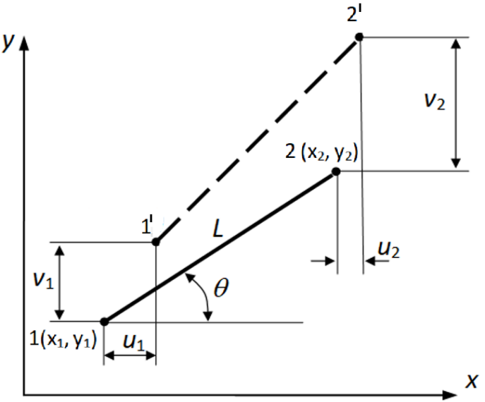
Figure 1. Initial and displaced configurations of a two-node truss element.
For initial nodal coordinates(x1,y1) and(x2,y2), the initial length is:
L=(x2−x1)2+(y2−y1)2
With element displacement vectoruel=(u1v1u2v2)T, the deformed length becomes:
Lf=(x2−x1+u2−u1)2+(y2−y1+v2−v1)2
The engineering axial strain, constant along the element, is:
Here, x1,x2,y1,y2 are the nodal coordinates, andu1,u2,v1,v2 are the corresponding nodal displacements.
03
Total potential energy
The total potential energy of the structure is the sum of the elastic deformation energy and the potential of the applied nodal forces. Here the applied loads are assumed to be conservative, displacement-independent nodal forces:
The summation extends over the deformation energy of all truss elements. Because the strain is constant along each element, the structural energy becomes:
Π=21el∑EALε2−uTF
Since the strain is constant within a truss element of cross-sectional area A,
Uel=21EALε2
The minimum-total-potential-energy principle requires
Ψ=∂u∂Π=∂u∂U−F=0
Substitution of the element energy gives the nonlinear system in the nodal displacements:
Ψ=el∑EALε∂u∂ε−F=0
04
Element force and tangent stiffness
At truss-element level, the deformation energy is:
In general, the element internal-force vector and tangent stiffness matrix are obtained as derivatives of the element energy:
fel=∂uel∂Uel,kel=∂uel∂fel=∂uel2∂2Uel
fel=EALε∂uel∂ε
kel=EAL[ε∂uel2∂2ε+∂uel∂ε(∂uel∂ε)T]
For the complete structure, assembly gives:
Kt=el∑kel,Ψ=el∑fel−F
The structural tangent matrix is the Hessian of the internal energy:
Kt=∂u2∂2Π=∂u2∂2U=∂u2∂2(∑elUel)
Assembly
The global tangent matrix is assembled using the same connectivity procedure as in a linear finite element model. The nonlinearity enters through the displacement-dependent element quantities.
05
Newton–Raphson solution
The nonlinear algebraic systemΨ=0 is solved iteratively. At iterationi,
Δu(i)=−(Kt(i))−1Ψ(i)u(i+1)=u(i)+Δu(i)
A displacement-based convergence measure is:
η=nΔuTΔu<tol
where n is the number of active equations.
Important remark
The method is exact within the stated assumptions. Its accuracy does not depend on the number of load steps. Buckling of individual truss elements is not considered.
06
MATLAB implementation
The following symbolic MATLAB program computesfel andkel as derivatives of Uel.
k_sym.mSymbolic derivation
% k_symclearsyms x1 x2 u1 u2 y1 y2 v1 v2 L EA real
U=EA/2/L*(sqrt((x2-x1+u2-u1)^2+(y2-y1+v2-v1)^2)-L)^2;
fel=[diff(U,u1); diff(U,v1); diff(U,u2); diff(U,v2)];
fel=simplify(fel)
kel=[diff(fel,u1) diff(fel,v1) diff(fel,u2) diff(fel,v2)];
kel=simplify(kel)
The resulting expressions are copied into thestiff.m subroutine. The nonlinear analysis is started by running main.m, which calls:
gen.m — generates the numerical input data;
stiff.m — assembles and solves the nonlinear system iteratively;
strain_stress.m — computes strains and stresses in all truss elements.
The Newton–Raphson update in stiff.m is implemented as
Direct differentiation ofε=Lf/L−1 gives the exact gradient and Hessian:
∂uel∂ε=LLf1a,∂uel2∂2ε=LLf1G−LLf31aaT
For very small axial deformation, one may set Lf≈L. The additional approximation∂2ε/∂uel2≈(1/L2)G omits the second term of the exact Hessian:
∂uel∂ε≈L21a,∂uel2∂2ε≈L21G
This is a computational approximation, not the exact second derivative obtained merely by substitutingLf=L. The supplied deriv.m uses the exact expressions, while retaining their compact form.
Tested in MATLAB R2017b and MATLAB R2026a. The derivative checks passed, all nonlinear solvers converged, the linear solution remained finite, and the two equivalent nonlinear implementations agreed to machine precision. The programs use standard MATLAB syntax and are expected to be compatible with intermediate and newer MATLAB versions.
07
Numerical examples
Example 1 — vertical loading
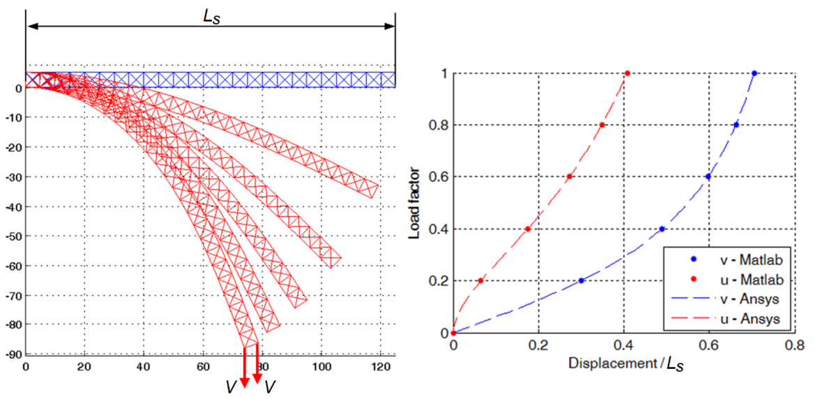
The complete numerical input data are given ingen.m. A vertical loadV=100N is applied at the free end. The deformed configurations and load–displacement curves show the strongly nonlinear geometric response of the structure.
Figure 2. Deformed configurations and comparison of MATLAB and ANSYS load–displacement results.
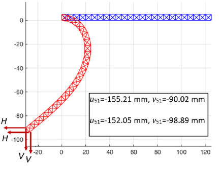
Example 2 — combined horizontal and vertical loading
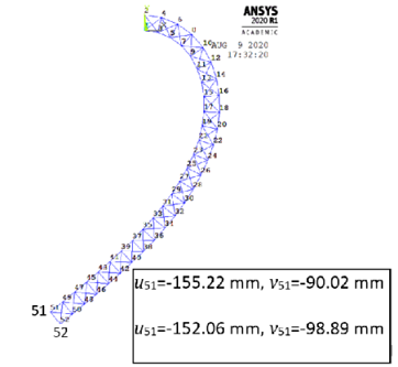
A horizontal load H=200N is added to the vertical loadV=100N. The MATLAB and ANSYS displacement results are identical to the displayed precision.
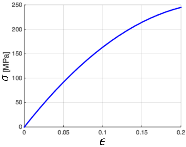
In Example 3, some element strains exceed 10%, so the small-strain material interpretation is no longer appropriate. In the formulation below,ε is engineering strain andσ is its work-conjugate nominal stress. If the relation is supplied as a nonlinear functionσ=f(ε), the elastic strain-energy density is the area under the stress–strain curve. Therefore,
Uel=AL∫0εσ(ξ)dξ
The function σ(ε) is assumed to be known experimentally. Differentiation gives the consistent internal-force vector:
fel=ALσ(ε)∂uel∂ε
With the material tangentEt=dσ/dε, the consistent element tangent is:
kel=AL[Et∂uel∂ε(∂uel∂ε)T+σ∂uel2∂2ε]
Figure 4. Tabulated nonlinear stress–strain relation used in the example.
The tangent ∂σ/∂ε is computed from the same shape-preserving interpolation used for the tabulated stress–strain relation. The program uses this material tangent together with the exact strain Hessian, so the assembled matrix is consistent with the internal-force vector.
Scope of Example 3
In this example, the strains are large and the material response is nonlinear.