16.1. Isoparametric 4-node quadrilateral

Corotational principle

StrainSmall

DisplacementLarge

MaterialLinear elastic

Stress statePlane stress

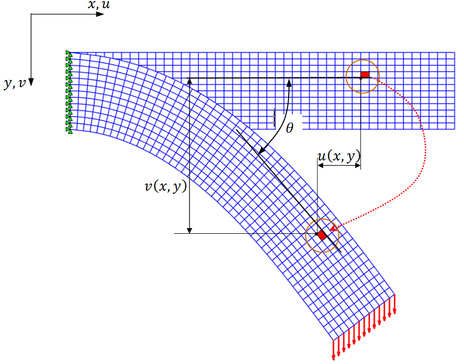
A finite element can undergo large displacements while its strains remain small; consequently, its dimensions remain practically unchanged. The displacement can be regarded as the sum of two parts: a large rigid-body motion, consisting of a finite translation and a large rotation, and a small displacement that produces deformation.

The usual engineering strain definition is not suitable when a finite rigid-body rotation is present. The translation disappears when displacement derivatives are evaluated, but the finite rotation would produce large parasitic strains and stresses. Chapter 10 introduced Green–Lagrange strain to remove this problem. The corotational formulation provides another approach: it removes the rigid-body motion while retaining the engineering definition of strain for the small deformational part.

\left\{\begin{aligned}\varepsilon_x&=\frac{\partial u}{\partial x}\\[4pt]\varepsilon_y&=\frac{\partial v}{\partial y}\\[4pt]\gamma_{xy}&=\frac{\partial u}{\partial y}+\frac{\partial v}{\partial x}\end{aligned}\right.

\boldsymbol{x}=\left\{\begin{matrix}x\\[-3pt]y\end{matrix}\right\},\qquad \boldsymbol{u}=\left\{\begin{matrix}u\\[-3pt]v\end{matrix}\right\}

Large deformation of a plane-stress cantilever with rigid-body rotation and displacement components — **Figure 1.** Large displacement of the structure, showing the rigid-body translation and rotation together with the small deformational part.

Initial, current, and corotational configurations

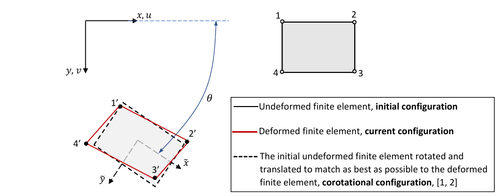
The rigid-body motion consists of a translation and a finite rotation. The rigid translation does not need to be introduced explicitly in the subsequent strain equations because it is constant over the element and therefore disappears when the displacement derivatives are taken.

The nodal coordinates of the undeformed initial finite-element configuration are denoted by $\boldsymbol{x}_{el0}$ . The nodal coordinates of the current deformed element are:

\boldsymbol{x}_{el}=\boldsymbol{x}_{el0}+\boldsymbol{u}_{el}

where $\boldsymbol{u}_{el}$ contains the nodal displacements.

We seek a representative rigid-body rotation that makes the initial element configuration match the current configuration as closely as possible, so that the remaining corotational displacements correspond mainly to the small deformational part. In the simple approach used here, the signed rotations of the four homologous sides are computed and their arithmetic average is taken as the element rigid-body rotation. Consequently, the nodal coordinates of the corotational configuration are:

\widetilde{\boldsymbol{x}}_{el}=\boldsymbol{R}\boldsymbol{x}_{el0}

with:

\boldsymbol{R}=\begin{bmatrix}\cos\theta&\sin\theta\\-\sin\theta&\cos\theta\end{bmatrix}

The corotational nodal displacements used in the subsequent computation are:

\widetilde{\boldsymbol{u}}_{el}=\boldsymbol{x}_{el}-\widetilde{\boldsymbol{x}}_{el}\qquad\text{or}\qquad\widetilde{\boldsymbol{u}}_{el}=\boldsymbol{x}_{el0}+\boldsymbol{u}_{el}-\boldsymbol{R}\boldsymbol{x}_{el0}\qquad\text{or}\qquad\widetilde{\boldsymbol{u}}_{el}=(\boldsymbol{I}_2-\boldsymbol{R})\boldsymbol{x}_{el0}+\boldsymbol{u}_{el}

Finite-element equations

The problem is nonlinear; therefore, the following system of nonlinear equations must be solved, using the notation introduced in Section 12.2:

\boldsymbol{\Psi}\left(\boldsymbol{u}\right)=\mathcal{A}_{el=1}^{n_{el}}\!\left(h\sum_{n_G}\boldsymbol{B}^{T}\boldsymbol{\sigma}\det(\boldsymbol{J})\right)-\boldsymbol{F}=\boldsymbol{0}\qquad\text{or}\qquad\boldsymbol{\Psi}\left(\boldsymbol{u}\right)=\mathcal{A}_{el=1}^{n_{el}}\!\left(\boldsymbol{f}_{el}\right)-\boldsymbol{F}=\boldsymbol{0}

Here, $\mathcal{A}$ denotes the standard finite-element assembly operator. The element internal-force vector is:

\boldsymbol{f}_{el}=h\sum_{n_G}\boldsymbol{B}^{T}\boldsymbol{\sigma}\det(\boldsymbol{J})\qquad\text{or}\qquad\boldsymbol{f}_{el}=h\sum_{n_G}\boldsymbol{B}^{T}\boldsymbol{D}\boldsymbol{B}\widetilde{\boldsymbol{u}}_{el}\det(\boldsymbol{J})

Here, $h$ denotes the initial element thickness. In the numerical implementation, the current thickness is updated to account for transverse contraction, as shown below.

In the present approach, the stiffness matrix of one finite element is approximated by:

\boldsymbol{k}_{el}=\frac{\partial\boldsymbol{f}_{el}}{\partial\widetilde{\boldsymbol{u}}_{el}}\approx h\sum_{n_G}\boldsymbol{B}^{T}\frac{\partial\boldsymbol{\sigma}}{\partial\widetilde{\boldsymbol{u}}_{el}}\det(\boldsymbol{J})=h\sum_{n_G}\boldsymbol{B}^{T}\boldsymbol{D}\boldsymbol{B}\det(\boldsymbol{J})

This expression is similar to the linear formulation presented in Section 9.4, but the corotational displacement $\widetilde{\boldsymbol{u}}_{el}$ is used instead of $\boldsymbol{u}_{el}$ . In addition, $\boldsymbol{B}$ and $\boldsymbol{J}$ are evaluated from the current coordinates $\boldsymbol{x}_{el}=\boldsymbol{x}_{el0}+\boldsymbol{u}_{el}$ , rather than from $\boldsymbol{x}_{el0}$ . This makes the problem nonlinear.

The strains are computed from derivatives of the corotational displacements:

\left\{\begin{aligned}\varepsilon_x&=\frac{\partial\widetilde{u}}{\partial x}\\[4pt]\varepsilon_y&=\frac{\partial\widetilde{v}}{\partial y}\\[4pt]\gamma_{xy}&=\frac{\partial\widetilde{u}}{\partial y}+\frac{\partial\widetilde{v}}{\partial x}\end{aligned}\right.

The difference $\widetilde{\boldsymbol{u}}-\boldsymbol{u}=\left(\boldsymbol{I}_2-\boldsymbol{R}\right)\boldsymbol{x}_0$ is considered constant within the element. The displacements $\boldsymbol{u}$ and $\widetilde{\boldsymbol{u}}$ at a point are interpolated from the nodal displacements by the shape functions $N(s,t)$ introduced in Section 9.4. The derivatives are evaluated in the global reference frame for the current configuration.

MATLAB implementation

With these specifications, the stiff routine from Section 9.4 can be adapted to solve the nonlinear large-displacement problem. The essential sequence is:

rot
for j=1:4
    s=st(1,j);
    t=st(2,j);
    H=[(1+t)/4  -(1+t)/4  -(1-t)/4  (1-t)/4
       (1+s)/4   (1-s)/4  -(1-s)/4 -(1+s)/4];
    J=H*[xdel ydel];                  % Jacobian
    detJ=abs(det(J));
    J1=inv(J);
    b=J1*H;

    % strain-displacement matrix
    B=[b(1,1)       0    b(1,2)       0    b(1,3)       0    b(1,4)       0
           0    b(2,1)       0    b(2,2)       0    b(2,3)       0    b(2,4)
       b(2,1)   b(1,1)   b(2,2)   b(1,2)   b(2,3)   b(1,3)   b(2,4)   b(1,4)];

    strn=B*sel;                        % strains
    th1=(1-nu/(1-nu)*(strn(1)+strn(2)))*th;
    fel=fel+th1*(B'*DHooke*strn)*detJ;
    kel=kel+th1*(B'*DHooke*B)*detJ;
    strnt(ig,:,istep)=strn';
    sigmt(ig,1:3,istep)=strn'*DHooke;
end

The rot routine computes the element rigid-body rotation $\theta$ , the current and corotational nodal coordinates, and the corotational nodal displacements. The correspondence between the theoretical notation and MATLAB variables is:

Theoretical quantity	MATLAB implementation
$\boldsymbol{x}_{el0}$	`xel, yel`
$\boldsymbol{x}_{el}=\boldsymbol{x}_{el0}+\boldsymbol{u}_{el}$	`xdel, ydel`
$\widetilde{\boldsymbol{x}}_{el}=\boldsymbol{R}\boldsymbol{x}_{el0}$	`xyr=R*[xel yel]'`
$\widetilde{\boldsymbol{u}}_{el}=\boldsymbol{x}_{el}-\boldsymbol{R}\boldsymbol{x}_{el0}$	`sel=[xdel ydel]'-xyr`

The main differences between the linear routine plane2d from Section 9.4 and the nonlinear routine stiff are summarized below.

Linear program	Nonlinear program — large displacements
`J=H*[xel yel];` The nodal displacements are $\boldsymbol{u}_{el}$	`J=H[xdel ydel];` `strn=Bsel`; the nodal displacements `sel` represent $\widetilde{\boldsymbol{u}}_{el}$
The equations are written for the initial undeformed configuration of the structure.	The equations are written for the current deformed configuration of the structure.

Rigid-body rotation and thickness update

For each side $i$ , $\boldsymbol{d}_i^0$ denotes the side vector in the initial undeformed configuration, and $\boldsymbol{d}_i^c$ denotes the corresponding side vector in the current deformed configuration. The signed rotation used in the present rotation-matrix convention is:

\theta_i=\operatorname{atan2}\!\left[(\boldsymbol{d}_i^c\times\boldsymbol{d}_i^0)_z,\,\boldsymbol{d}_i^c\cdot\boldsymbol{d}_i^0\right]

Using atan2 instead of asin removes the ambiguity associated with determining the angle from its sine only, because both the cross-product and dot-product information are used.

for i=1:4
    i1=mod(i,4)+1;
    dxy =[xel(i1)-xel(i)   yel(i1)-yel(i)   0];
    dxyd=[xdel(i1)-xdel(i) ydel(i1)-ydel(i) 0];

    cr=cross(dxyd,dxy);
    dt=dot(dxyd,dxy);
    thet(i)=atan2(cr(3),dt);
end

thetm=mean(thet);

The arithmetic average of the four signed side rotations is retained:

\boxed{\theta=\frac{1}{4}\left(\theta_{12}+\theta_{23}+\theta_{34}+\theta_{41}\right)}

Both the linear analysis of Section 9.4 and the nonlinear analysis presented here are performed in the global reference frame, and both use the engineering definition of strain. Because the nonlinear analysis is performed on the current deformed configuration, it produces Cauchy stresses. The current thickness is updated to account for transverse contraction:

h\longrightarrow h_1=h\left[1-\frac{\nu}{1-\nu}(\varepsilon_x+\varepsilon_y)\right]

Important remark. The corotational formulation presented here is not incremental with respect to the strain or reference configuration. The converged final solution does not depend on the number of load steps. Load stepping may nevertheless be used to facilitate convergence or to follow the response of the structure during loading, for example to obtain a force–displacement curve. If only the final state is required and convergence is achieved, a single load step gives the same final result.

Example 1

A cantilever beam of length $L=400\,\mathrm{mm}$ , with a rectangular cross-section of thickness $5\,\mathrm{mm}$ and height $20\,\mathrm{mm}$ , has material properties $E=1000\,\mathrm{MPa}$ and $\nu=0.3$ . A force $F=100\,\mathrm{N}$ is applied at the free end. The mesh contains 60 elements along the length and 8 elements through the height: 480 4-node isoparametric elements, 549 nodes, and 8 load steps.

Axial Cauchy stress on the deformed cantilever at load step 8 — **Figure 3.** Axial Cauchy stress $\sigma_x$ at load step 8.

UL formulation — Euler–Almansi strain

$u_{\min}=-155.59\,\mathrm{mm}\qquad u_{\max}=2.44\,\mathrm{mm}$

$v_{\min}=-286.49\,\mathrm{mm}\qquad v_{\max}=0$

$\sigma_{x,\min}=-83.38\,\mathrm{MPa}\qquad \sigma_{x,\max}=73.60\,\mathrm{MPa}$

CR formulation — engineering strain

$u_{\min}=-155.72\,\mathrm{mm}\qquad u_{\max}=2.39\,\mathrm{mm}$

$v_{\min}=-286.45\,\mathrm{mm}\qquad v_{\max}=0$

$\sigma_{x,\min}=-81.55\,\mathrm{MPa}\qquad \sigma_{x,\max}=75.19\,\mathrm{MPa}$

ANSYS

$u_{\min}=-155.68\,\mathrm{mm}\qquad u_{\max}=2.352\,\mathrm{mm}$

$v_{\min}=-286.32\,\mathrm{mm}\qquad v_{\max}=0$

$\sigma_{x,\min}=-79.78\,\mathrm{MPa}\qquad \sigma_{x,\max}=76.96\,\mathrm{MPa}$

The UL and CR formulations give nearly identical displacements, while the stresses differ by about 2% at the clamped end, where the stresses are maximum and the axial strain is approximately 7%. The value of about 7% is already rather high for the small-strain assumption, but it is strongly localized in the immediate vicinity of the clamped end.

Both UL and CR produce Cauchy stresses because the analysis is performed on the deformed current structure.

Tangent-stiffness approximation

The element internal-force vector is:

\boldsymbol{f}_{el}=h\sum_{n_G}\boldsymbol{B}^{T}\boldsymbol{\sigma}\det(\boldsymbol{J})

In the present formulation, the stiffness matrix is approximated by:

\boldsymbol{k}_{el}=\frac{\partial\boldsymbol{f}_{el}}{\partial\widetilde{\boldsymbol{u}}_{el}}=\frac{\partial}{\partial\widetilde{\boldsymbol{u}}_{el}}\!\left(h\sum_{n_G}\boldsymbol{B}^{T}\boldsymbol{\sigma}\det(\boldsymbol{J})\right)\approx h\sum_{n_G}\boldsymbol{B}^{T}\frac{\partial\boldsymbol{\sigma}}{\partial\widetilde{\boldsymbol{u}}_{el}}\det(\boldsymbol{J})=h\sum_{n_G}\boldsymbol{B}^{T}\boldsymbol{D}\boldsymbol{B}\det(\boldsymbol{J})

The internal nodal force vector $\boldsymbol{f}_{el}$ is evaluated consistently for the current configuration. The stiffness matrix $\boldsymbol{k}_{el}$ , however, is only an approximation to the exact tangent matrix, because the dependence of both $\boldsymbol{B}$ and $\boldsymbol{J}$ on the current nodal displacements is neglected. The equilibrium equations can nevertheless be solved iteratively and the procedure converges, but the approximate tangent generally leads to slower convergence. Section 16.2 shows how the tangent matrix can be improved by including these neglected terms.

An underrelaxation factor $s_r$ may be introduced in the main program:

sr=0.5;
for istep=1:nstep
    error=1;
    iter=0;
    while (error > tol) & (iter < itermax)
        iter=iter+1;
        stiff
        dS=K\F*sr;
        S=S-dS;
        error=sqrt(dS'*dS/n);
    end
end

Comparison of TL, UL, and CR formulations

A concise comparison of the three formulations is given below [1].

Total Lagrangian formulation (TL)

The finite-element equations are formulated with respect to the initial fixed reference configuration, which does not change throughout the analysis; see Section 12.2.

Updated Lagrangian formulation (UL)

The reference is the last known accepted solution. It is kept fixed over a load step and updated at the end of each load step; see Sections 15.2 and 15.3.

Corotational formulation (CR)

The finite-element equations of each element are referred to two configurations. The initial undeformed configuration is used, as in TL, to compute the element rigid-body motion. The current deformed state is then referred to the corotational configuration obtained by applying that rigid-body motion to the initial reference configuration.

A detailed treatment of the CR formulation is given in [2]; the present section develops a simple plane-stress implementation.

Program and download

A MATLAB program package for this example can be downloaded below. Run main.m.

MMATLAB packageDOWNLOAD ZIP

References

Lagrangian and Corotational Formulations, Altair, 2021.
Felippa, C. A., Nonlinear Finite Element Methods, Department of Aerospace Engineering Sciences, University of Colorado at Boulder, Chapters 12 and 13, 2004.