15.4. Comparison between TL and UL formulations

Overview

This section presents a comparison between the Total Lagrangian (TL) and Updated Lagrangian (UL) formulations using two examples. Loads that produce relatively high strains are considered to highlight important differences between the formulations.

Example 1

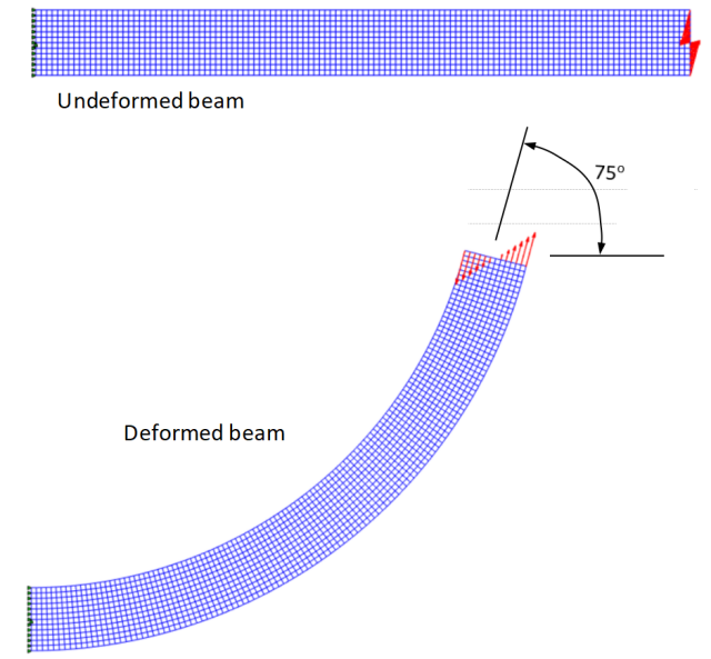
A cantilever beam of length $L=400\,\mathrm{mm}$ , with a rectangular cross-section of thickness $5\,\mathrm{mm}$ and height $40\,\mathrm{mm}$ , has material properties $E=1000\,\mathrm{MPa}$ and $\nu=0.3$ . A moment $C=87500\,\mathrm{Nmm}$ is applied at the free end. The mesh has 120 elements along the length and 12 elements through the height: 1440 4-node isoparametric elements and 1573 nodes.

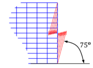
The boundary constraints and loading are shown below. The forces that produce the moment $C$ have a fixed direction and form a constant angle of $75^\circ$ with the horizontal. They are represented on both the initial undeformed configuration and the final deformed beam.

To obtain a pure-bending state in the section of interest, only the horizontal displacements are constrained at the left end.

Finite element mesh and boundary constraints at the clamped end — **Figure 1.** Boundary constraints, loading, and deformed configuration for Example 1.

Undeformed beam, loading direction, and final deformed configuration — **Figure 1.** Boundary constraints, loading, and deformed configuration for Example 1.

Example 1: beam-theory estimates

The bending angle is:

\varphi=\frac{CL}{EI}=\frac{87500\cdot400}{1000\left(40^3\cdot5/12\right)}=1.31\,\mathrm{rad}=75^\circ

The maximum axial stress is:

\sigma_{\max}=\frac{C}{W}=\frac{87500}{40^2\cdot5/6}=65.63\,\mathrm{MPa}

The maximum axial strain is approximately:

\varepsilon_x\approx0.07

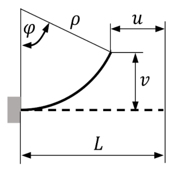
Assuming that the neutral axis bends into a circular arc, its radius of curvature is (see Section 15.2):

Circular-arc geometry used to estimate the cantilever tip displacements — **Figure 2.** Circular-arc geometry and beam-theory estimates for the cantilever tip displacements.

Example 1: TL and UL results

Total Lagrangian (TL)	Updated Lagrangian (UL)
Non-incremental presentation on this site. Reference configuration: initial undeformed configuration.	Incremental approach. Reference configuration: current configuration.
Green–Lagrange strains Second Piola–Kirchhoff stresses	Euler–Almansi strains Cauchy stresses
Displacements of the midpoint of the free-end section and maximum axial stress
$u=-106.74\,\mathrm{mm}$ $v=-228.88\,\mathrm{mm}$ $\sigma_{x,\max}=66.8\,\mathrm{MPa}$	$u=-105.58\,\mathrm{mm}$ $v=-227.84\,\mathrm{mm}$ $\sigma_{x,\max}=64.2\,\mathrm{MPa}$

TL axial PK2 stress on the initial reference configuration — **Figure 3.** The axial PK2 stress $S_x$ is shown on the initial reference configuration in the global frame $(x,y)$ .

Global coordinate axes — **Figure 3.** The axial PK2 stress $S_x$ is shown on the initial reference configuration in the global frame $(x,y)$ .

UL axial Cauchy stress on the current reference configuration — **Figure 4.** The axial Cauchy stress $\sigma_x$ is shown on the current reference configuration in the global frame $(x,y)$ .

PK2 stress plotted on the deformed beam geometry — **Figure 5.** Here, the PK2 stress $S_x$ is plotted on the deformed beam geometry.

Cauchy stress plotted on the deformed beam geometry with the inclined local reference frame — **Figure 6.** Here, the Cauchy stress $\bar{\sigma}_x$ is plotted on the deformed beam geometry in the local reference frame $(\bar{x},\bar{y})$ .

\bar{\boldsymbol\sigma}=\boldsymbol R\boldsymbol\sigma\boldsymbol R^T

\boldsymbol\sigma=\begin{bmatrix}\sigma_x&\tau_{xy}\\\tau_{xy}&\sigma_y\end{bmatrix}\qquad \bar{\boldsymbol\sigma}=\begin{bmatrix}\bar\sigma_x&\bar\tau_{xy}\\\bar\tau_{xy}&\bar\sigma_y\end{bmatrix}\qquad \boldsymbol R=\begin{bmatrix}\cos\theta&\sin\theta\\-\sin\theta&\cos\theta\end{bmatrix}

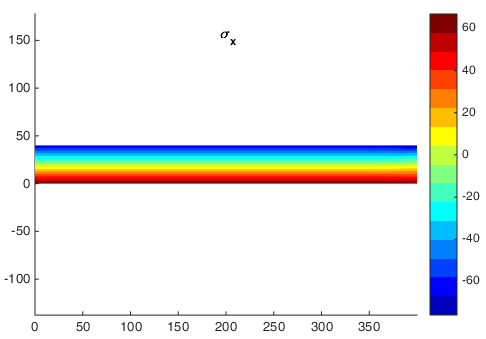
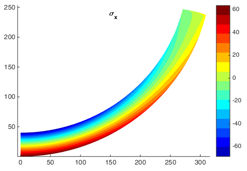
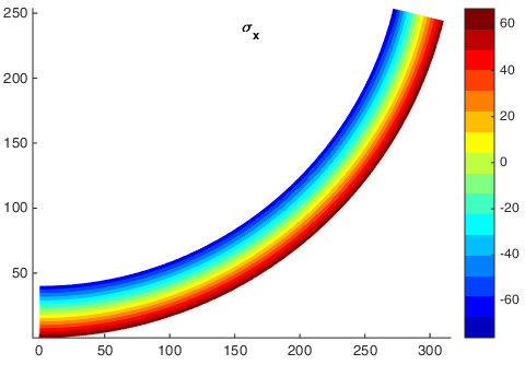
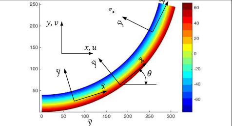
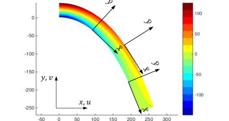
The local reference frame $\bar{x}\bar{y}$ is obtained by rotating the global $xy$ frame until the local $\bar{x}$ -axis becomes tangent to the deformed beam fiber passing through the point considered. The local $\bar{y}$ -axis is normal to this tangent.

The MATLAB subprogram plot_stress_r rotates the stress components with respect to the local reference frame. The program is available in the download section below.

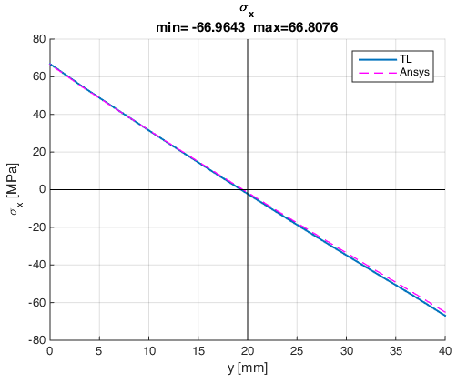
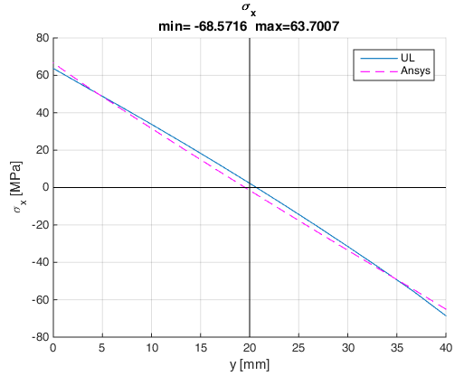
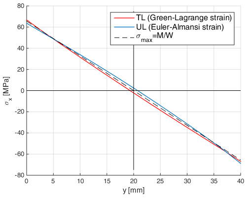
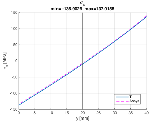
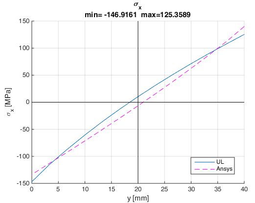
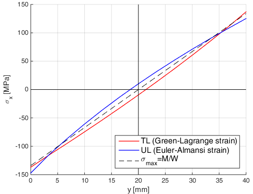
TL and ANSYS axial stress distributions across the clamped section — **Figure 7.** TL and ANSYS results.

UL and ANSYS axial stress distributions across the clamped section — **Figure 8.** UL and ANSYS results.

The axial-stress distributions obtained with TL and UL are compared with the linear result from classical beam theory:

Comparison of TL, UL, and linear beam-theory axial stress distributions — **Figure 9.** $\sigma_x$ stress distribution within the cross section at the clamped end.

Example 2

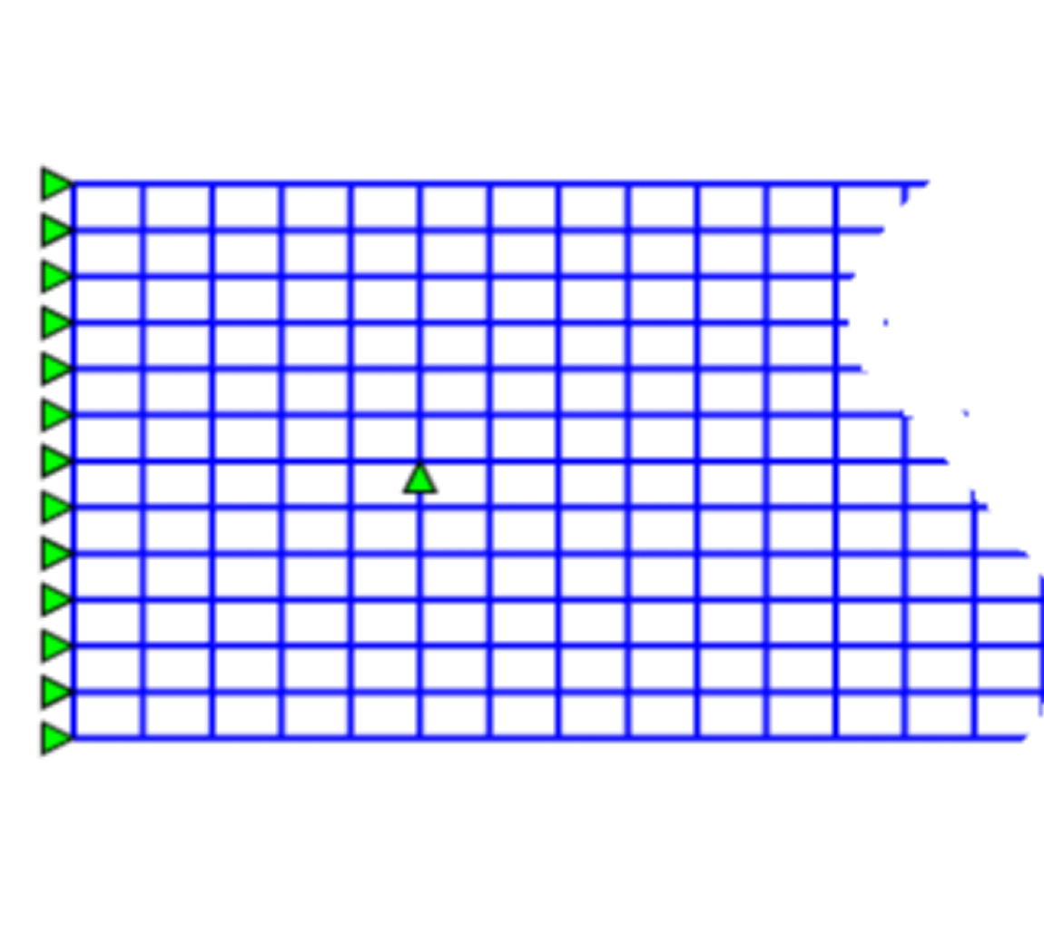
A cantilever beam of length $L=400\,\mathrm{mm}$ , with a rectangular cross-section of thickness $5\,\mathrm{mm}$ and height $40\,\mathrm{mm}$ , has material properties $E=1000\,\mathrm{MPa}$ and $\nu=0.3$ . A force $F=800\,\mathrm{N}$ is applied at the free end. The mesh has 80 elements along the length and 12 elements through the height: 960 4-node isoparametric elements and 1053 nodes.

A single vertical support is placed sufficiently far from this section so that it does not disturb the stress state there.

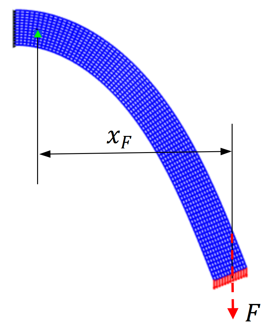
Example 2 mesh and support arrangement — **Figure 10.** Boundary constraints, loading, and deformed configuration for Example 2.

Deformed beam, vertical load F, and horizontal distance x_F — **Figure 10.** Boundary constraints, loading, and deformed configuration for Example 2.

The bending moment in the section considered is $M=F x_F$ , where $x_F$ is the horizontal distance to the vertical support.

The maximum axial stress from beam theory is:

\sigma_{\max}=\frac{F x_F}{W}=\frac{1.7867\times10^5}{40^2\cdot5/6}=134\,\mathrm{MPa}

The maximum axial strain is approximately:

\varepsilon_x\approx0.135

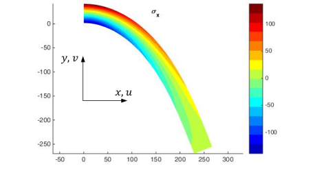
Example 2: TL and UL results

Total Lagrangian (TL)	Updated Lagrangian (UL)
Green–Lagrange strains Second Piola–Kirchhoff stresses	Euler–Almansi strains Cauchy stresses
Non-incremental presentation on this site. Reference configuration: initial undeformed configuration.	Incremental approach. Reference configuration: current configuration.
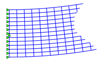
Displacements of the midpoint of the free-end section
$u=-151.94\,\mathrm{mm}$ $v=282.36\,\mathrm{mm}$	$u=-151.45\,\mathrm{mm}$ $v=282.38\,\mathrm{mm}$

TL axial PK2 stress on the initial reference configuration for Example 2 — **Figure 11.** The axial PK2 stress $S_x$ is shown on the initial reference configuration in the global frame $(x,y)$ .

UL axial Cauchy stress on the current reference configuration for Example 2 — **Figure 12.** The axial Cauchy stress $\sigma_x$ is shown on the current reference configuration in the global frame $(x,y)$ .

TL axial PK2 stress on the deformed current geometry for Example 2 — **Figure 13.** Here, the PK2 stress $S_x$ is plotted on the deformed beam geometry.

UL axial Cauchy stress in the local frame on the deformed geometry for Example 2 — **Figure 14.** Here, the Cauchy stress $\bar{\sigma}_x$ is plotted on the deformed beam geometry in the local reference frame $(\bar{x},\bar{y})$ .

\bar{\boldsymbol\sigma}=\boldsymbol R\boldsymbol\sigma\boldsymbol R^T

TL and ANSYS axial stress distributions across the clamped section in Example 2 — **Figure 15.** TL and ANSYS results.

UL and ANSYS axial stress distributions across the clamped section in Example 2 — **Figure 16.** UL and ANSYS results.

Large-strain comparison

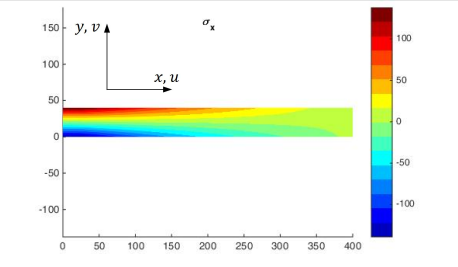
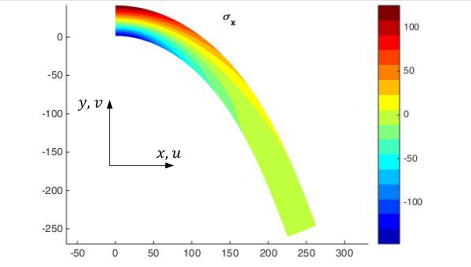
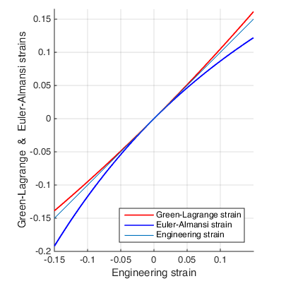
The TL and UL stress distributions are quite different from the linear one because the maximum strain is large, about $0.135=13.5\%$ . Their shapes are consistent with the behavior of the Green–Lagrange and Euler–Almansi strain measures shown in Chapter 13, Figure 1.

If the strain $\varepsilon\in[-0.05,0.05]$ , the differences between engineering strain and the other two measures are about 2–3% for Green–Lagrange strain and around 7% for Euler–Almansi strain. For steel, for example, the maximum axial strain $\varepsilon$ is usually smaller than 0.01 if no plasticity occurs, so the value of 0.135 used in this example is intentionally very large in order to make the effects of the different strain measures clearly visible.

TL, UL, and linear beam-theory axial stress distributions for Example 2 — **Figure 17.** $\sigma_x$ stress distribution within the cross section at the clamped end.

Green-Lagrange, Euler-Almansi, and engineering strain comparison from Chapter 13 — **Figure 18.** Green–Lagrange, Euler–Almansi, and engineering strains.

Program and download

The MATLAB subprogram used to rotate the stress components into the local reference frame can be downloaded below.

MMATLAB subprogramDownload ZIP