UL formulation: plane stress, isoparametric 4-node quadrilateral, Hencky strain, improved approach

01

Formulation and hypotheses

Section 17.2 introduced a simple UL formulation using Hencky or Biot strains, together with an approximate tangent stiffness matrix. The present section keeps the same strain measures and the same strain–displacement matrix $\boldsymbol{B}$, but improves the tangent stiffness by retaining additional geometric terms. The aim is to obtain better convergence without changing the equilibrium equation itself.

Let us first consider the Biot strains (see Section 17.1).

02

Biot strain and deformation gradient

In the case of small strains, it can be written:

$\varepsilon_x,\varepsilon_y,\gamma_{xy}$ are the engineering strains. The deformation gradient is (see Chapter 10):

03

Q4 displacement derivatives

For the isoparametric quadrilateral finite element, the displacement derivatives are (see Sections 9.4 and 12.2):

with:

$\boldsymbol{u}_{el}$ contains the nodal displacements of the current finite element:

Therefore:

and:

04

Engineering strain relations

It is easy to show that for small quantities:

or:

It results:

Or in engineering notation:

These equations are the same as those obtained in Section 12.2:

where:

$\boldsymbol{G}_x,\boldsymbol{G}_y,\boldsymbol{G}_{xy}$ are symmetric $8\times8$ matrices.

It is worth noting that the equations containing the matrices $\boldsymbol{G}_x$, $\boldsymbol{G}_y$, and $\boldsymbol{G}_{xy}$ are identical to those obtained in Chapter 12 for the Green–Lagrange strain formulation.

05

Improved stiff subprogram

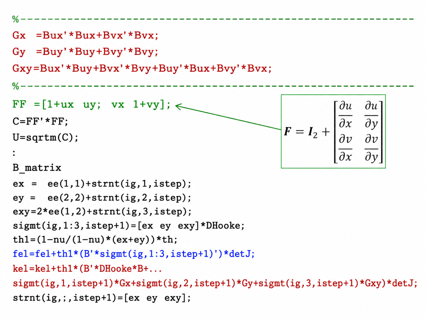
Only a few changes must be made in the stiff subprogram given in Section 17.2. The lines shown in red were added or modified in the new stiff subprogram, as illustrated below:

Recall that the following equation (see the blue line in Figure 1) is exact:

$h_1$ is the current finite-element thickness, which accounts for the thickness modification due to transverse contraction (see Section 15.1):

The strain–displacement matrix $\boldsymbol{B}$ is the same matrix derived in Section 17.2 and is computed, for each element and Gauss point, by the same B_matrix subroutine. In the program, B_matrix is called before the computation of the element internal force vector $\boldsymbol{f}_{el}$ and tangent stiffness matrix $\boldsymbol{k}_{el}$. The improvement introduced here concerns the tangent stiffness matrix, not the definition or computation of $\boldsymbol{B}$.

Compared with the expression used in Section 17.2, the tangent stiffness matrix becomes:

Therefore, the additional geometric terms significantly improve convergence.

Everything explained in this section also applies to Hencky strains because the strains are small:

06

Strain update and reference-configuration correction

During the iterations corresponding to load step $i+1$, the strains are updated:

Neither the Hencky strain tensor nor the Biot strain tensor is generally additive under finite successive deformations. In the present small-strain UL formulation, the update $\boldsymbol{e}_{i+1}\approx\boldsymbol{e}_{i}+\Delta\boldsymbol{e}$ is therefore only an incremental approximation.

A formulation that avoids this approximate additive accumulation by updating the deformation gradient multiplicatively is presented in Section 17.4: UL formulation with multiplicative update of the deformation gradient.

The terms $\boldsymbol{e}_{i}$ and $\Delta\boldsymbol{e}$ are calculated for the configuration at load step $i$, while $\boldsymbol{e}_{i+1}$ must be calculated for the slightly different configuration corresponding to load step $i+1$. This error decreases as the number of load steps increases. Another method for correcting this error is described in Section 15.2.

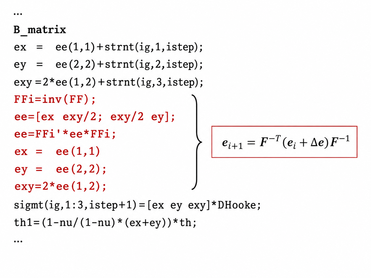
To account for the fact that $\boldsymbol{e}_{i}$ and $\Delta\boldsymbol{e}$ are evaluated with respect to slightly different configurations, the strain tensor is transferred to the current configuration before the stresses are evaluated. The stiff subroutine therefore includes the following correction:

The deformation gradient $\boldsymbol{F}$ is already calculated to obtain the right stretch tensor $\boldsymbol{U}$; see the green line in Figure 1. In the final stiff subprogram, the red lines shown below are included:

As in Section 17.2, the same stiff subroutine can be used with either Hencky or Biot strains by setting istrain=1 or istrain=2.

07

Numerical example

Example. Consider a cantilever beam of length $L=400\ \mathrm{mm}$, with a rectangular cross-section of thickness $5\ \mathrm{mm}$ and height $20\ \mathrm{mm}$. The material properties are $E=1000\ \mathrm{MPa}$ and $\nu=0.3$. The free end is loaded by a force $F=100\ \mathrm{N}$. The mesh contains $60\times8=480$ 4-node isoparametric elements and 549 nodes. The load is applied in 20 steps.

The table below shows that the reference-configuration correction significantly improves the results, even for a small number of load steps.

08

Programs and download

The modified MATLAB programs can be downloaded below.