Isoparametric 8-node hexahedral finite element

01

Introduction

The 8-node hexahedral finite element is the 3D counterpart of the 4-node quadrilateral element presented in Section 15.3. The corresponding linear formulation is briefly described in Section 25.1. The Updated Lagrangian (UL) formulation has already been introduced in Chapter 15 and will not be repeated here.

As in the 2D case, the configuration at the beginning of each load increment is taken as the updated reference configuration. The HEX8 element has three displacement degrees of freedom per node and uses $2^3=8$ Gauss integration points.

02

Direct evaluation of Euler–Almansi strain

Following Sections 15.3 and 15.4, the total deformation gradient is evaluated directly from the initial and current trial configurations:

Here $\htmlClass{fea-math-bold-italic}{\boldsymbol J}_0$ and $\htmlClass{fea-math-bold-italic}{\boldsymbol J}_t$ denote the Jacobians in the initial and current trial configurations. Thus, the total Euler–Almansi strain is obtained without accumulating strain components over successive increments.

This approach uses the MATLAB routine stiff.m when use_mult=false.

J0=H*[xel0 yel0 zel0];
Jt=H*[xelt yelt zelt];
Ftot=(J0\Jt)';
btens=Ftot*Ftot';
ee=0.5*(eye(3)-inv(btens));

03

Multiplicative update of the deformation gradient

Alternatively, the total deformation gradient can be updated from the preceding converged configuration instead of referring to the initial configuration at every iteration. At each Gauss point, the incremental deformation gradient and the total gradient in the trial configuration are:

Here $\htmlClass{fea-math-bold-italic}{\boldsymbol F}_n$ is the total deformation gradient stored at the end of the preceding converged load increment. Initially, $\htmlClass{fea-math-bold-italic}{\boldsymbol F}_0=\htmlClass{fea-math-bold-italic}{\boldsymbol I}$ at every Gauss integration point. During Newton–Raphson iterations, $\htmlClass{fea-math-bold-italic}{\boldsymbol F}_n$ remains fixed while the trial $\htmlClass{fea-math-bold-italic}{\boldsymbol F}_t$ is recomputed. After convergence, the last evaluated $\htmlClass{fea-math-bold-italic}{\boldsymbol F}_t$ is stored for use in the next load increment.

Jt=H*[xelt yelt zelt];
Finc=(J\Jt)';
Ftot=Finc*Fhist(:,:,ig);
Ftotsal(:,:,ig)=Ftot;
btens=Ftot*Ftot';
ee=0.5*(eye(3)-inv(btens));

In main.m, the Gauss-point history is initialized by Fhist=repmat(eye(3),[1 1 8*nel]) and, after convergence, updated by Fhist=Ftotsal. The alternative stiff_mult.m replaces the direct evaluation when use_mult=true; use_mult=false selects stiff.m. Both routines use the same internal-force and stiffness expressions.

04

Incremental stiffness and equilibrium

As in Section 15.3, the strain-displacement matrix $\htmlClass{fea-math-bold-italic}{\boldsymbol B}$ and the stiffness expressions retain the incremental Green–Lagrange construction (using the matrices $\htmlClass{fea-math-bold-italic}{\boldsymbol G}_x$, $\htmlClass{fea-math-bold-italic}{\boldsymbol G}_y$, $\htmlClass{fea-math-bold-italic}{\boldsymbol G}_z$, $\htmlClass{fea-math-bold-italic}{\boldsymbol G}_{xy}$, $\htmlClass{fea-math-bold-italic}{\boldsymbol G}_{yz}$ and $\htmlClass{fea-math-bold-italic}{\boldsymbol G}_{zx}$), while stresses are calculated from the directly evaluated Euler–Almansi strain. The relevant program statements are:

B0=[Bux; Bvy; Bwz; Buy+Bvx; Bvz+Bwy; Bwx+Buz];
BL=[sel'*Gx; sel'*Gy; sel'*Gz; sel'*Gxy; sel'*Gyz; sel'*Gzx];
B=B0+BL;
sigmt(ig,1:6,istep+1)=[ex ey ez exy eyz ezx]*DHooke;
fel=fel+(B'*sigmt(ig,1:6,istep+1)')*detJ;

The element tangent matrix is assembled as the material contribution $\htmlClass{fea-math-bold-italic}{\boldsymbol B}^T\htmlClass{fea-math-bold-italic}{\boldsymbol D}\htmlClass{fea-math-bold-italic}{\boldsymbol B}$ plus six stress-dependent geometric contributions ($\htmlClass{fea-math-bold-italic}{\boldsymbol G}_x,\htmlClass{fea-math-bold-italic}{\boldsymbol G}_y,\htmlClass{fea-math-bold-italic}{\boldsymbol G}_z,\htmlClass{fea-math-bold-italic}{\boldsymbol G}_{xy},\htmlClass{fea-math-bold-italic}{\boldsymbol G}_{yz},\htmlClass{fea-math-bold-italic}{\boldsymbol G}_{zx}$), as shown in the downloadable MATLAB program.

This mixed formulation is an approximation intended to keep the implementation simple under the small-strain assumption. Its accuracy can be assessed by load-increment refinement; a fully consistent spatial residual and tangent matrix will be considered in Section 27.2.

05

Example

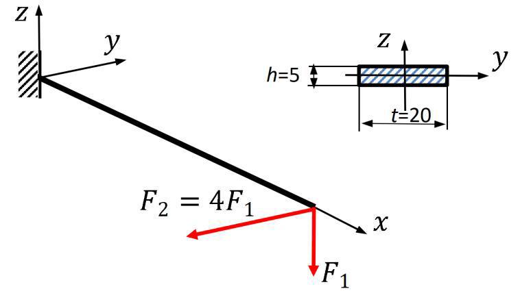
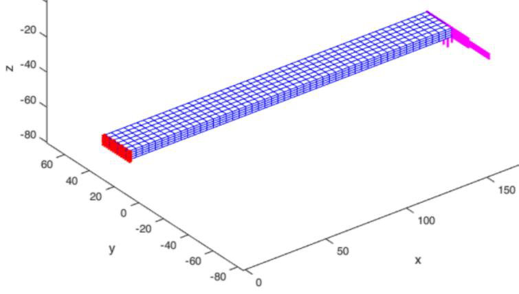
A straight cantilever of length $L=200\,\mathit{mm}$ and rectangular cross-section $t=20\,\mathit{mm},\ h=5\,\mathit{mm}$ is subjected to the end loads $F_1=20\,\mathit N$ and $F_2=4F_1$. The material constants are $E=1000\,\mathit{MPa}$ and $\nu=0.3$. The mesh consists of $50\times6\times4=1200$ HEX8 elements, 1785 nodes and 5355 displacement degrees of freedom.

06

Numerical results

The displacement response of the center of the loaded cross-section agrees closely with the ANSYS results, as shown in Figure 2. For this diagram, the analysis used 50 load increments.

The longitudinal Cauchy stress $\sigma_x$ at load step 50 is shown in Figure 3. The plotted values range from $-70.46$ to $101.57\,\mathit{MPa}$.

07

Load-increment sensitivity

The final extrema of the vertical displacement $w$, computed with different numbers of load increments, are:

The difference in $|w_{\mathop{\mathit{min}}}|$ between 20 and 50 increments is approximately 0.044%, indicating low sensitivity to further load-increment refinement in this example. The supplied MATLAB main program uses nstep = 20 by default; set nstep = 50 to reproduce Figures 2 and 3.

08

MATLAB program

The MATLAB package contains both stiff.m and stiff_mult.m. Run main.m; select the direct or multiplicative approach using use_mult.

09

Interactive 3D figure

An interactive visualization of the longitudinal stress $\sigma_x$ follows. The model can be rotated and enlarged; Reset view restores its initial orientation.