01
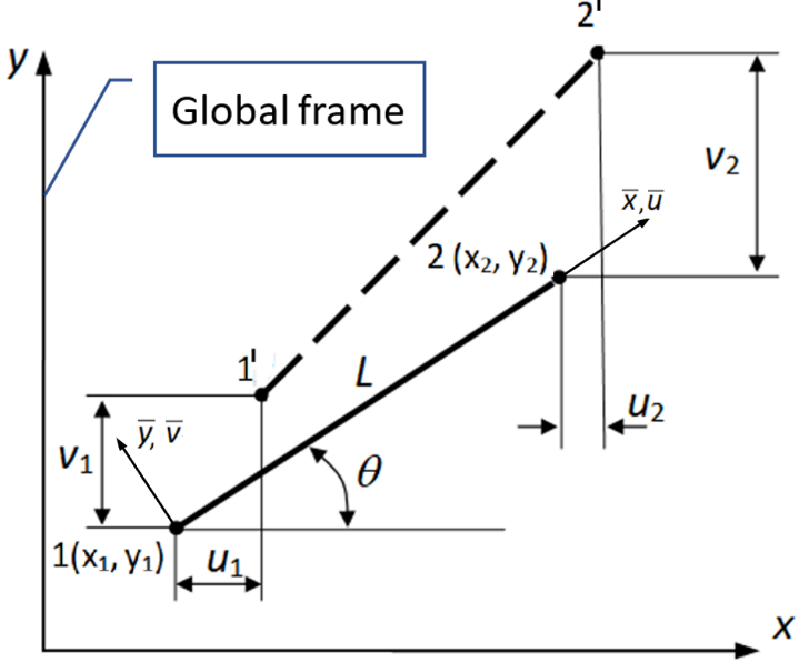
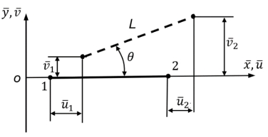
Local reference frame Consider a two-node truss element under the hypotheses of small displacements, small strains, and linear elastic material behaviour.
The element is initially inclined at an angleθ \theta θ x y xy x y x ˉ \bar{x} x ˉ
02
Second-order axial strain As established in Section 1.1, the exact engineering strain in global coordinates is:
ε = ( x 2 − x 1 + u 2 − u 1 L ) 2 + ( y 2 − y 1 + v 2 − v 1 L ) 2 − 1 \varepsilon=\sqrt{\left(\frac{x_2-x_1+u_2-u_1}{L}\right)^2+\left(\frac{y_2-y_1+v_2-v_1}{L}\right)^2}-1 ε = ( L x 2 − x 1 + u 2 − u 1 ) 2 + ( L y 2 − y 1 + v 2 − v 1 ) 2 − 1 Equivalently,
ε = ( cos θ + u 2 − u 1 L ) 2 + ( sin θ + v 2 − v 1 L ) 2 − 1 \varepsilon=\sqrt{\left(\cos\theta+\frac{u_2-u_1}{L}\right)^2+\left(\sin\theta+\frac{v_2-v_1}{L}\right)^2}-1 ε = ( cos θ + L u 2 − u 1 ) 2 + ( sin θ + L v 2 − v 1 ) 2 − 1 In the local frame,x ˉ 2 − x ˉ 1 = L \bar{x}_2-\bar{x}_1=L x ˉ 2 − x ˉ 1 = L y ˉ 2 − y ˉ 1 = 0 \bar{y}_2-\bar{y}_1=0 y ˉ 2 − y ˉ 1 = 0
ε = ( 1 + u ˉ 2 − u ˉ 1 L ) 2 + ( v ˉ 2 − v ˉ 1 L ) 2 − 1 \varepsilon=\sqrt{\left(1+\frac{\bar{u}_2-\bar{u}_1}{L}\right)^2+\left(\frac{\bar{v}_2-\bar{v}_1}{L}\right)^2}-1 ε = ( 1 + L u ˉ 2 − u ˉ 1 ) 2 + ( L v ˉ 2 − v ˉ 1 ) 2 − 1 ε = 1 + 2 u ˉ 2 − u ˉ 1 L + ( u ˉ 2 − u ˉ 1 ) 2 L 2 + ( v ˉ 2 − v ˉ 1 ) 2 L 2 − 1 \varepsilon=\sqrt{1+2\frac{\bar{u}_2-\bar{u}_1}{L}+\frac{(\bar{u}_2-\bar{u}_1)^2}{L^2}+\frac{(\bar{v}_2-\bar{v}_1)^2}{L^2}}-1 ε = 1 + 2 L u ˉ 2 − u ˉ 1 + L 2 ( u ˉ 2 − u ˉ 1 ) 2 + L 2 ( v ˉ 2 − v ˉ 1 ) 2 − 1 The barred displacements are measured in the local reference frame. Introduce
a = 2 u ˉ 2 − u ˉ 1 L + ( u ˉ 2 − u ˉ 1 ) 2 L 2 + ( v ˉ 2 − v ˉ 1 ) 2 L 2 a=2\frac{\bar{u}_2-\bar{u}_1}{L}+\frac{(\bar{u}_2-\bar{u}_1)^2}{L^2}+\frac{(\bar{v}_2-\bar{v}_1)^2}{L^2} a = 2 L u ˉ 2 − u ˉ 1 + L 2 ( u ˉ 2 − u ˉ 1 ) 2 + L 2 ( v ˉ 2 − v ˉ 1 ) 2 For ∣ a ∣ ≪ 1 |a|\ll1 ∣ a ∣ ≪ 1 [1]
1 + a = 1 + 1 2 a − 1 8 a 2 + 1 16 a 3 − 5 128 a 4 + 7 256 a 5 − ⋯ \sqrt{1+a}=1+\frac{1}{2}a-\frac{1}{8}a^2+\frac{1}{16}a^3-\frac{5}{128}a^4+\frac{7}{256}a^5-\cdots 1 + a = 1 + 2 1 a − 8 1 a 2 + 16 1 a 3 − 128 5 a 4 + 256 7 a 5 − ⋯ Retaining the first three terms gives:
1 + a ≈ 1 + 1 2 a − 1 8 a 2 \sqrt{1+a}\approx1+\frac{1}{2}a-\frac{1}{8}a^2 1 + a ≈ 1 + 2 1 a − 8 1 a 2 After neglecting terms of degree three and higher in the nodal displacements, the second-order strain is:
ε ≈ u ˉ 2 − u ˉ 1 L + ( v ˉ 2 − v ˉ 1 ) 2 2 L 2 \varepsilon\approx\frac{\bar{u}_2-\bar{u}_1}{L}+\frac{(\bar{v}_2-\bar{v}_1)^2}{2L^2} ε ≈ L u ˉ 2 − u ˉ 1 + 2 L 2 ( v ˉ 2 − v ˉ 1 ) 2 04
Element deformation energy For one linear elastic truss element,
U e l = 1 2 E A L ε 2 U_{el}=\frac{1}{2}EAL\varepsilon^2 U e l = 2 1 E A L ε 2 Substituting the second-order strain and neglecting the fourth-degree term gives:
U e l ≈ 1 2 E A L ε 0 2 + 1 2 E A L ε 0 u ˉ e l T C ˉ u ˉ e l U_{el}\approx\frac{1}{2}EAL\varepsilon_0^2+\frac{1}{2}EAL\varepsilon_0\bar{\boldsymbol{u}}_{el}^{T}\bar{\boldsymbol{C}}\bar{\boldsymbol{u}}_{el} U e l ≈ 2 1 E A L ε 0 2 + 2 1 E A L ε 0 u ˉ e l T C ˉ u ˉ e l U e l = 1 2 u ˉ e l T k ˉ e l u ˉ e l + 1 2 u ˉ e l T k ˉ G , e l u ˉ e l U_{el}=\frac{1}{2}\bar{\boldsymbol{u}}_{el}^{T}\bar{\boldsymbol{k}}_{el}\bar{\boldsymbol{u}}_{el}+\frac{1}{2}\bar{\boldsymbol{u}}_{el}^{T}\bar{\boldsymbol{k}}_{G,el}\bar{\boldsymbol{u}}_{el} U e l = 2 1 u ˉ e l T k ˉ e l u ˉ e l + 2 1 u ˉ e l T k ˉ G , e l u ˉ e l or
U e l = 1 2 u ˉ e l T ( k ˉ e l + k ˉ G , e l ) u ˉ e l = 1 2 u ˉ e l T k ˉ t o t a l , e l u ˉ e l U_{el}=\frac{1}{2}\bar{\boldsymbol{u}}_{el}^{T}\left(\bar{\boldsymbol{k}}_{el}+\bar{\boldsymbol{k}}_{G,el}\right)\bar{\boldsymbol{u}}_{el}=\frac{1}{2}\bar{\boldsymbol{u}}_{el}^{T}\bar{\boldsymbol{k}}_{\mathrm{total},el}\bar{\boldsymbol{u}}_{el} U e l = 2 1 u ˉ e l T ( k ˉ e l + k ˉ G , e l ) u ˉ e l = 2 1 u ˉ e l T k ˉ total , e l u ˉ e l Because the displacements are small, the axial force is evaluated from the first-order strain
N = E A ε 0 N=EA\varepsilon_0 N = E A ε 0 05
Stiffness matrices in the local frame The elastic stiffness matrix is:
k ˉ e l = E A L B ˉ T B ˉ = E A L { − 1 0 1 0 } { − 1 0 1 0 } T \bar{\boldsymbol{k}}_{el}=EAL\bar{\boldsymbol{B}}^{T}\bar{\boldsymbol{B}}=\frac{EA}{L}\begin{Bmatrix}-1\\0\\1\\0\end{Bmatrix}\begin{Bmatrix}-1\\0\\1\\0\end{Bmatrix}^{T} k ˉ e l = E A L B ˉ T B ˉ = L E A ⎩ ⎨ ⎧ − 1 0 1 0 ⎭ ⎬ ⎫ ⎩ ⎨ ⎧ − 1 0 1 0 ⎭ ⎬ ⎫ T k ˉ e l = E A L [ 1 0 − 1 0 0 0 0 0 − 1 0 1 0 0 0 0 0 ] \bar{\boldsymbol{k}}_{el}=\frac{EA}{L}\begin{bmatrix}1&0&-1&0\\0&0&0&0\\-1&0&1&0\\0&0&0&0\end{bmatrix} k ˉ e l = L E A 1 0 − 1 0 0 0 0 0 − 1 0 1 0 0 0 0 0 The geometric stiffness matrix is:
k ˉ G , e l = N L C ˉ = N L { 0 1 0 − 1 } { 0 1 0 − 1 } T \bar{\boldsymbol{k}}_{G,el}=NL\bar{\boldsymbol{C}}=\frac{N}{L}\begin{Bmatrix}0\\1\\0\\-1\end{Bmatrix}\begin{Bmatrix}0\\1\\0\\-1\end{Bmatrix}^{T} k ˉ G , e l = N L C ˉ = L N ⎩ ⎨ ⎧ 0 1 0 − 1 ⎭ ⎬ ⎫ ⎩ ⎨ ⎧ 0 1 0 − 1 ⎭ ⎬ ⎫ T k ˉ G , e l = N L [ 0 0 0 0 0 1 0 − 1 0 0 0 0 0 − 1 0 1 ] \bar{\boldsymbol{k}}_{G,el}=\frac{N}{L}\begin{bmatrix}0&0&0&0\\0&1&0&-1\\0&0&0&0\\0&-1&0&1\end{bmatrix} k ˉ G , e l = L N 0 0 0 0 0 1 0 − 1 0 0 0 0 0 − 1 0 1 This energy-based separation into elastic and geometric contributions is the standard stress-stiffening construction [2] [3]
06
Transformation to the global frame For an element inclined at angleθ \theta θ
u ˉ e l = R u e l \bar{\boldsymbol{u}}_{el}=\boldsymbol{R}\boldsymbol{u}_{el} u ˉ e l = R u e l R = [ c s 0 0 − s c 0 0 0 0 c s 0 0 − s c ] c = cos θ s = sin θ \boldsymbol{R}=\begin{bmatrix}c&s&0&0\\-s&c&0&0\\0&0&c&s\\0&0&-s&c\end{bmatrix}\qquad c=\cos\theta\qquad s=\sin\theta R = c − s 0 0 s c 0 0 0 0 c − s 0 0 s c c = cos θ s = sin θ The total element stiffness matrix is therefore:
k t o t a l , e l = R T k ˉ t o t a l , e l R \boldsymbol{k}_{\mathrm{total},el}=\boldsymbol{R}^{T}\bar{\boldsymbol{k}}_{\mathrm{total},el}\boldsymbol{R} k total , e l = R T k ˉ total , e l R k e l + k G , e l = R T ( k ˉ e l + k ˉ G , e l ) R \boldsymbol{k}_{el}+\boldsymbol{k}_{G,el}=\boldsymbol{R}^{T}\left(\bar{\boldsymbol{k}}_{el}+\bar{\boldsymbol{k}}_{G,el}\right)\boldsymbol{R} k e l + k G , e l = R T ( k ˉ e l + k ˉ G , e l ) R In the global frame, the elastic stiffness matrix is:
k e l = E A L [ c 2 c s − c 2 − c s c s s 2 − c s − s 2 − c 2 − c s c 2 c s − c s − s 2 c s s 2 ] \boldsymbol{k}_{el}=\frac{EA}{L}\begin{bmatrix}c^2&cs&-c^2&-cs\\cs&s^2&-cs&-s^2\\-c^2&-cs&c^2&cs\\-cs&-s^2&cs&s^2\end{bmatrix} k e l = L E A c 2 cs − c 2 − cs cs s 2 − cs − s 2 − c 2 − cs c 2 cs − cs − s 2 cs s 2 k e l = E A L { − cos θ − sin θ cos θ sin θ } { − cos θ − sin θ cos θ sin θ } T \boldsymbol{k}_{el}=\frac{EA}{L}\begin{Bmatrix}-\cos\theta\\-\sin\theta\\\cos\theta\\\sin\theta\end{Bmatrix}\begin{Bmatrix}-\cos\theta\\-\sin\theta\\\cos\theta\\\sin\theta\end{Bmatrix}^{T} k e l = L E A ⎩ ⎨ ⎧ − cos θ − sin θ cos θ sin θ ⎭ ⎬ ⎫ ⎩ ⎨ ⎧ − cos θ − sin θ cos θ sin θ ⎭ ⎬ ⎫ T The geometric stiffness matrix is:
k G , e l = N L [ s 2 − c s − s 2 c s − c s c 2 c s − c 2 − s 2 c s s 2 − c s c s − c 2 − c s c 2 ] \boldsymbol{k}_{G,el}=\frac{N}{L}\begin{bmatrix}s^2&-cs&-s^2&cs\\-cs&c^2&cs&-c^2\\-s^2&cs&s^2&-cs\\cs&-c^2&-cs&c^2\end{bmatrix} k G , e l = L N s 2 − cs − s 2 cs − cs c 2 cs − c 2 − s 2 cs s 2 − cs cs − c 2 − cs c 2 k G , e l = N L { − sin θ cos θ sin θ − cos θ } { − sin θ cos θ sin θ − cos θ } T \boldsymbol{k}_{G,el}=\frac{N}{L}\begin{Bmatrix}-\sin\theta\\\cos\theta\\\sin\theta\\-\cos\theta\end{Bmatrix}\begin{Bmatrix}-\sin\theta\\\cos\theta\\\sin\theta\\-\cos\theta\end{Bmatrix}^{T} k G , e l = L N ⎩ ⎨ ⎧ − sin θ cos θ sin θ − cos θ ⎭ ⎬ ⎫ ⎩ ⎨ ⎧ − sin θ cos θ sin θ − cos θ ⎭ ⎬ ⎫ T These are the same elastic and geometric stiffness matrices obtained directly in global coordinates in Section 1.2.
07
Verification Independent matrix check
Both identitiesk e l = R T k ˉ e l R \boldsymbol{k}_{el}=\boldsymbol{R}^{T}\bar{\boldsymbol{k}}_{el}\boldsymbol{R} k e l = R T k ˉ e l R k G , e l = R T k ˉ G , e l R \boldsymbol{k}_{G,el}=\boldsymbol{R}^{T}\bar{\boldsymbol{k}}_{G,el}\boldsymbol{R} k G , e l = R T k ˉ G , e l R
No additional program package This section provides an alternative derivation of the matrices used in Section 1.2. It introduces no new MATLAB program, so there is no separate download package.
08
References Wikipedia contributors, “Binomial theorem” Ansys, Inc., Ansys Mechanical APDL Theory Reference I. Němec, M. Trcala, I. Ševčík, and H. Štekbauer, “New Formula for Geometric Stiffness Matrix Calculation” , Journal of Applied Mathematics and Physics , 4 (2016), 733–748. PREVIOUS SECTION ← 1.2. Buckling Analysis — Part I NEXT SECTION 2.1. Large Displacements of 3D Truss Structures →