01
Overview and assumptions
Consider a spatial structure assembled from straight, prismatic, two-node truss elements. Each element carries axial force only.
Notation
- Nodal-displacement vector in the global reference frame
- Nodal-force vector in the global reference frame
- Strain energy, potential of the applied forces, and total potential energy
- Axial stress and engineering strain
- Young's modulus, cross-sectional area, and initial element length
- Three-by-three identity matrix
02
Three-dimensional element kinematics
For the initial nodal coordinates and, the initial element length is:
Let be the displacement components of node. The deformed length is:
The engineering strain is therefore:
The six element degrees of freedom are collected in the column vector:
03
Total potential energy and equilibrium
For a linear elastic material,. The total potential energy of the assembled structure is:
Here , and the summation includes every truss element. The principle of minimum total potential energy requires
Substitution of the element energy gives:
Because the strain depends nonlinearly on the nodal displacements, these equilibrium equations are nonlinear.
04
Element internal force and tangent stiffness
The strain energy of one truss element is:
Differentiation with respect to the six element degrees of freedom gives the internal nodal-force vector and the consistent tangent stiffness matrix:
The order of the two gradient factors is important: their outer product is a matrix.
05
Exact strain derivatives
Introduce the deformed coordinate differences
and the compact quantities
The complete six-component strain gradient and the exact Hessian are:
When axial deformation is very small, the approximation may be used. This gives:
Replacing by does not by itself reduce the exact Hessian to. That shorter expression also omits the outer-product term. The supplied deriv.m uses the exact gradient and exact Hessian shown above.
06
Newton–Raphson solution and MATLAB implementation
At each iteration, the program assembles the structural tangent matrix and residual vector, applies the displacement constraints, and solves
% Exact engineering strain and derivatives
ep = Lf/L - 1;
q  = [dx+du; dy+dv; dz+dw];
a  = [-q; q];
G  = [eye(3) -eye(3); -eye(3) eye(3)];

ep1 = a/(L*Lf);
ep2 = G/(L*Lf) - (a*a')/(L*Lf^3);fel = EA*L*ep*ep1;
kel = EA*L*(ep*ep2 + ep1*ep1');
K(ip,ip) = K(ip,ip) + kel;
F(ip) = F(ip) + fel;Tested in MATLAB R2017b and MATLAB R2026a. Both versions produced the same displacement history and converged at all five load steps. The code uses standard MATLAB syntax and is expected to be compatible with intermediate and newer MATLAB versions.
07
Numerical example and ANSYS comparison
The example in gen.m contains 18 repeated spatial modules, 76 nodes, 234 truss elements, and 228 structural degrees of freedom. The complete load is applied in five equal steps.
At load step 4, the three displacement components of node 76 are compared below. The values are expressed in millimetres.
| Solution | |||
|---|---|---|---|
| MATLAB | 1760.9 | 2508.7 | −2639.6 |
| ANSYS | 1775.3 | 2520.0 | −2665.3 |
| Relative difference | 0.81% | 0.45% | 0.96% |
The agreement is close, with every reported component differing by less than 1%. The supplied ANSYS macro uses BEAM188 with a very small bending inertia to approximate an axial member; therefore, it is not mathematically identical to the pure truss model. ANSYS did not converge for the fifth load level, whereas the MATLAB program converged in seven iterations.
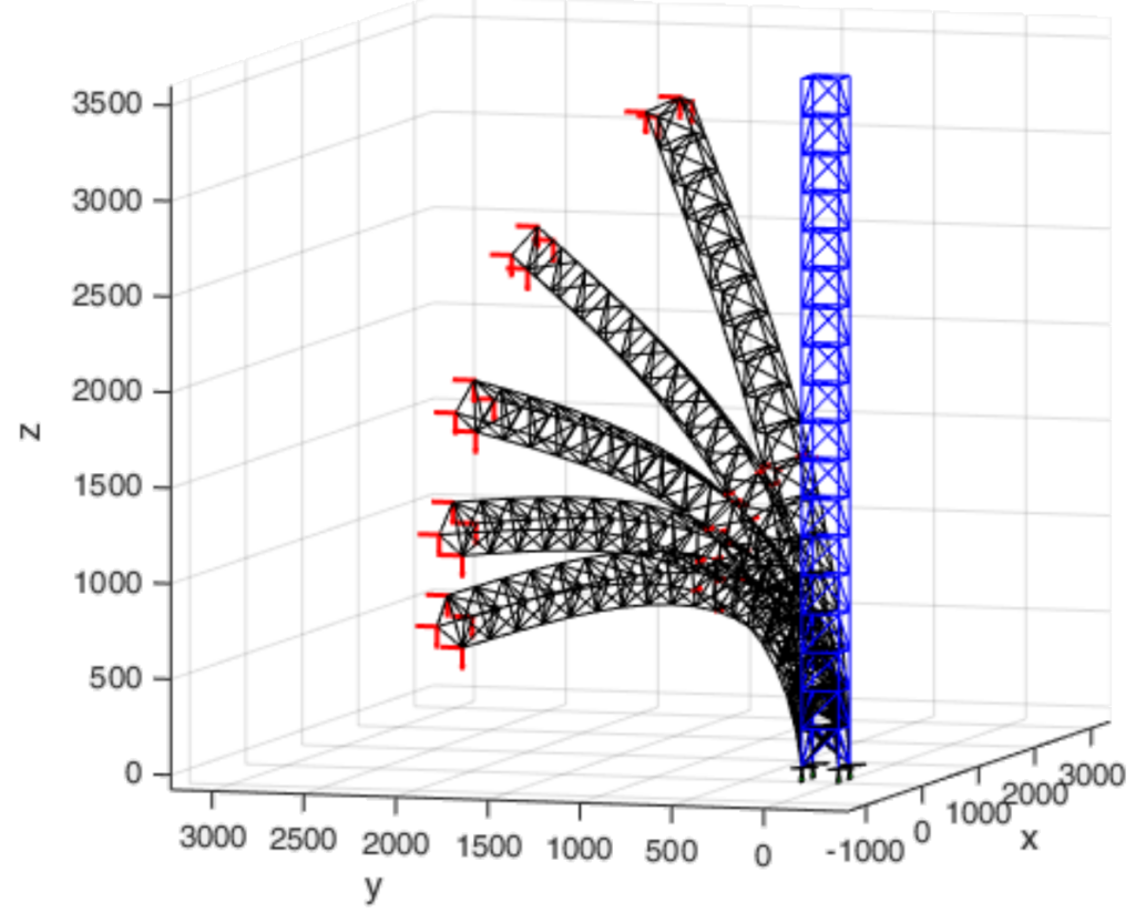
Within the stated assumptions, the formulation uses exact displacement kinematics and a consistent tangent. The number of load steps controls the numerical continuation path, not the converged equilibrium state. Local buckling of individual truss members is not included.
08
Program files
The MATLAB archive contains seven commented source files and a short README. The ANSYS macro is supplied separately so that the comparison model remains transparent.