01
Second-order axial strain
The analysis assumes small displacements, small strains, and a linear elastic material. Terms of second degree in the nodal displacements are nevertheless retained.
For the two-node spatial truss introduced in Section 2.1, the exact engineering strain is:
Let , , and be the direction cosines of the initial element axis. The same expression can be written as:
Using , define
Then
Although the displacements are small, the quadratic terms in , , and must be kept. The binomial expansion [1] is limited to its first three terms:
02
Compact matrix form
Neglecting terms of degree three and higher in all three displacement components gives:
where
If and , the same matrix has the compact form:
03
Element deformation energy
The deformation energy of one linear elastic truss element is:
Substitution of the second-order strain generates terms up to degree four. After neglecting the fourth-degree terms,
Since the displacements are small, the signed axial force from the preliminary linear analysis is:
Therefore,
04
Elastic and geometric stiffness matrices
Define the column vector:
The elastic stiffness matrix is:
The geometric stiffness matrix is:
The element matrices are assembled to obtain the structural elastic stiffness matrix and geometric stiffness matrix . This is the stress-stiffening contribution used in linearized eigenvalue buckling [2]
05
The buckling eigenproblem
Let the signed axial forces and correspond to a reference load. At a load factor , the total tangent stiffness becomes singular:
The MATLAB programs use in tension and in compression. The corresponding generalized eigenproblem is:
Here is the buckling load factor and is the buckling mode. Usually, only the smallest positive eigenvalue is required.
The minus sign follows directly from the determinant equation and from the signed axial-force convention used in the MATLAB files. It produces positive critical load factors for compression.
06
MATLAB implementation
The calculation is completed in two stages:
truss3d.msolves the small-displacement linear problem, andstress3d.mcomputes the signed axial forces in the trusses.buckling.massembles and computes the positive buckling load factors and their eigenvectors.
% Projection transverse to the element axis
direction = [dx;dy;dz]/L;
P = eye(3) - direction*direction';
kelG = (N(ie)/L)*[P -P;-P P];

% Compression is negative: K*phi = -lambda*KG*phi
[Vfree,D] = eig(Kff,-KGff);
lambdaAll = diag(D);Tested in MATLAB R2017b and MATLAB R2026a. Both versions returned the same four positive load factors. Restrained degrees of freedom are removed before solving, so nonphysical infinite eigenvalues are not included. The code uses standard MATLAB syntax and is expected to be compatible with intermediate and newer MATLAB versions.
07
Numerical example and ANSYS comparison
The data are defined in gen.m. The structure contains 18 repeated spatial modules, 76 nodes, 234 truss elements, and 228 degrees of freedom. A total reference load of 1 N acts downward at the four top nodes, so the numerical load factors also give the critical loads in newtons.
The four values computed with the MATLAB package are compared below with the ANSYS results.
| Mode | Verified MATLAB | ANSYS | Difference from ANSYS |
|---|---|---|---|
| 1 | 142,154.8729 N | 1.41923 × 10⁵ N | 0.163% |
| 2 | 158,603.4197 N | 1.5828 × 10⁵ N | 0.204% |
| 3 | 1,150,305.944 N | 1.1367 × 10⁶ N | 1.197% |
| 4 | 1,268,603.015 N | 1.2506 × 10⁶ N | 1.440% |
The supplied ANSYS macro uses BEAM188 with very small bending inertias to approximate axial members. It is therefore close to, but not mathematically identical with, the pure truss model used by MATLAB.
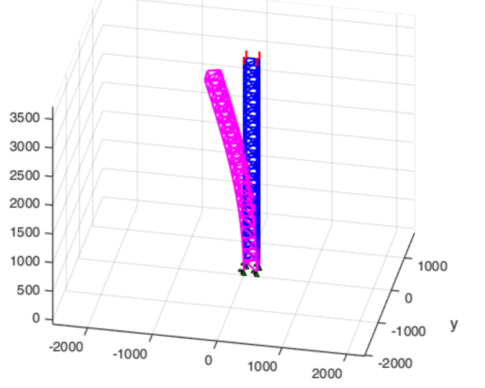
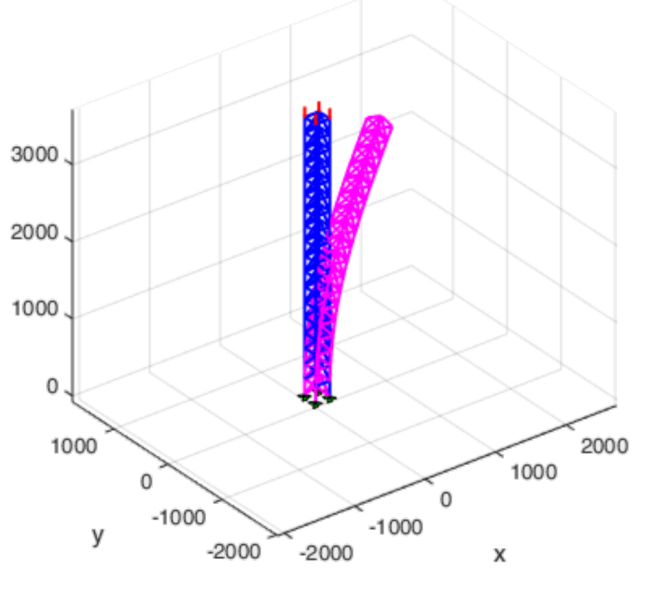
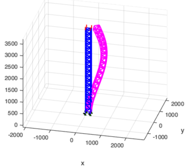
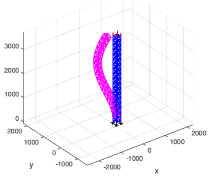
Figure 1. The first four buckling modes. The undeformed structure is blue and the scaled eigenvector is magenta.
08
Why the third binomial term matters
If the expansion is limited to only its first two terms,
the resulting strain is:
This expression is not the complete second-order expansion: orientation-dependent quadratic terms are lost. Its associated geometric stiffness matrix would be
This alternative matrix is invariant under rotation of the coordinate axes, but it is not algebraically equivalent to the consistent matrix obtained from the complete second-order expansion.
09
Program files
The MATLAB package contains six commented source files and a README. The ANSYS Mechanical APDL macro is supplied separately.
10
References
- Wikipedia contributors, “Binomial theorem”
- Ansys, Inc., Ansys Mechanical APDL Theory Reference, Release 2026 R1, sections “Stress Stiffening,” “Eigenvalue and Eigenvector Extraction,” and “Buckling Analysis,” 2026. The supplied comparison macro uses syntax compatible with ANSYS Release 12.0.