Large Displacements of a Cantilever Beam — Exact Solution

Model and assumptions

Consider a straight, prismatic cantilever of length $L$ and constant flexural rigidity $EI$ . Its free end is loaded by a force $P$ whose direction remains fixed.

MaterialLinear elastic

StrainSmall

DisplacementPotentially large

The Euler–Bernoulli model is used. Axial and shear deformations are neglected, so the centerline is inextensible and the cross-section remains normal to it.

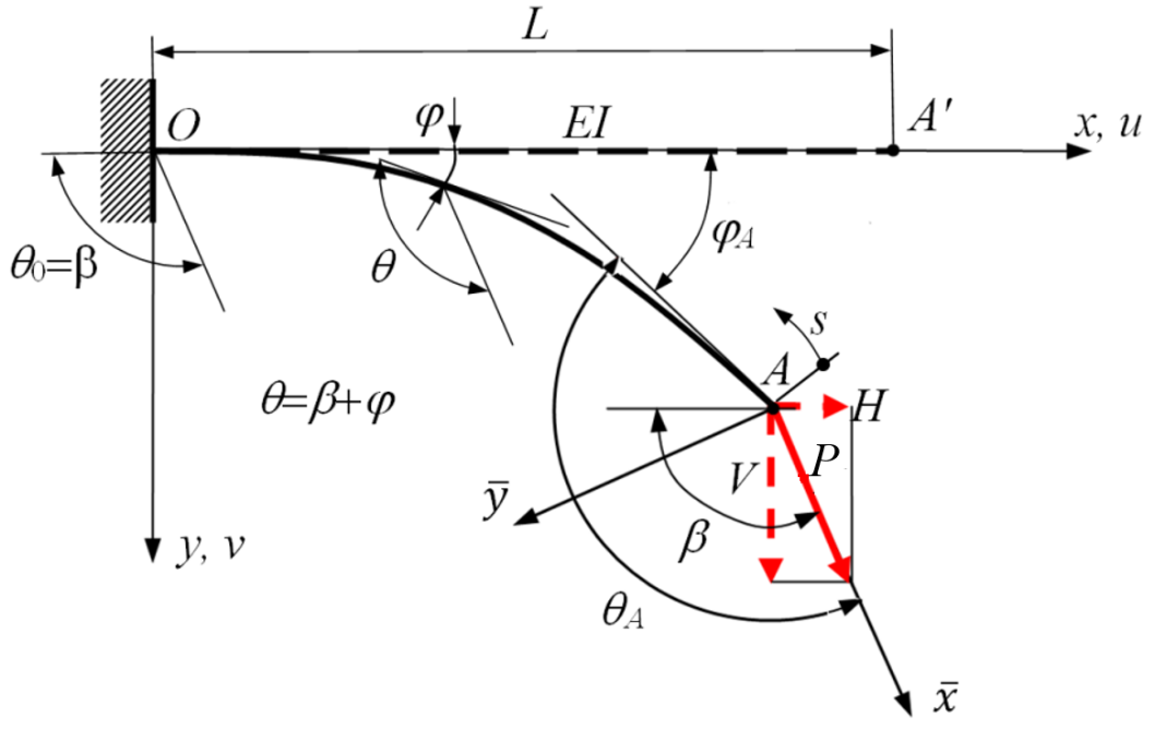
Cantilever elastica geometry, rotations, local axes, end-force components, and arc-length coordinate — Figure 1.Geometry and notation. The curvilinear coordinate $s_{AO}$ starts at the loaded end and increases toward the clamp.

Meaning of “exact”

The solution is exact within the stated Euler–Bernoulli, inextensible-centerline, linear-moment–curvature assumptions. It is not an exact three-dimensional elasticity solution.

The elastica differential equation

Let $\varphi$ be the cross-section rotation and $\beta$ the fixed force-direction angle. Define

\theta=\beta+\varphi

In the load-aligned local frame, $\bar{y}$ is the transverse distance from the force line through the free end. The bending moment and curvature satisfy

EI\kappa=M=-P\bar{y}

\kappa=\frac{d\varphi}{ds}=\frac{d\theta}{ds}

Because the centerline is inextensible,

\frac{d\bar{y}}{ds}=\sin\theta

Differentiating the moment–curvature equation gives the nonlinear pendulum equation for the planar elastica [1]

\frac{d^2\theta}{ds^2}=-\frac{P}{EI}\sin\theta

First integral and boundary conditions

At the free end $A$ , where $s=0$ , the bending moment and curvature vanish:

\theta(0)=\theta_A,\qquad \left.\frac{d\theta}{ds}\right|_{s=0}=0

Multiplying the differential equation by $d\theta/ds$ and integrating once gives:

\frac{1}{2}\left(\frac{d\theta}{ds}\right)^2=\frac{P}{EI}\left(\cos\theta-\cos\theta_A\right)

The integration constant is essential

The term $-\cos\theta_A$ follows from the zero-moment condition at the free end. Without it, the first integral does not satisfy the boundary condition from which the elliptic solution is obtained.

At the clamped end $O$ , where $s=L$ , the rotation is zero and therefore:

\theta(L)=\theta_0=\beta

Elliptic-integral solution

Following the elastica construction in [2], introduce

k=\sin\frac{\theta_A}{2},\qquad m=k^2

\sin\psi=\frac{\sin(\theta/2)}{k},\qquad \sin\psi_0=\frac{\sin(\beta/2)}{k}

At the free end, $\psi_A=\pi/2$ . The incomplete and complete elliptic integrals of the first kind are:

F(\psi,m)=\int_0^\psi\frac{d\alpha}{\sqrt{1-m\sin^2\alpha}},\qquad K(m)=F\left(\frac{\pi}{2},m\right)

The arc length measured from the free end is:

s=\sqrt{\frac{EI}{P}}\left[K(m)-F(\psi,m)\right]

Applying $s=L$ at the clamp gives the load–parameter relation:

P=\frac{EI}{L^2}\left[K(m)-F(\psi_0,m)\right]^2

This nonlinear scalar equation determines $m$ for prescribed $P$ and $\beta$ . On the principal real branch,

\sin^2\frac{\beta}{2}<m<1

Coordinates of the deformed beam

Define the incomplete and complete elliptic integrals of the second kind:

E(\psi,m)=\int_0^\psi\sqrt{1-m\sin^2\alpha}\,d\alpha,\qquad E(m)=E\left(\frac{\pi}{2},m\right)

In the local frame with origin at the loaded end, the exact centerline is:

\bar{x}=s\left[\frac{2\left(E(m)-E(\psi,m)\right)}{K(m)-F(\psi,m)}-1\right]

\bar{y}=\frac{2s\sqrt{m}\cos\psi}{K(m)-F(\psi,m)}

To place the clamp at the global origin, first translate the local coordinates:

\widetilde{x}(s)=\bar{x}(L)-\bar{x}(s),\qquad \widetilde{y}(s)=\bar{y}(L)-\bar{y}(s)

The coordinates plotted by the program are then

\begin{Bmatrix}x\\y\end{Bmatrix}=\begin{bmatrix}\cos\beta&\sin\beta\\\sin\beta&-\cos\beta\end{bmatrix}\begin{Bmatrix}\widetilde{x}\\\widetilde{y}\end{Bmatrix}

MATLAB implementation

Required toolbox

The programs use ellipticF, ellipticK, and ellipticE, which are provided by Symbolic Math Toolbox [3]. This toolbox is included in the current MATLAB and Simulink Home Suite. Users with other MATLAB license configurations should verify that Symbolic Math Toolbox is installed by entering ver in the Command Window.

The calculation has three parts:

findm.m finds the parameter $m$ by bisection on its physically admissible real interval.
main_cantilever.m evaluates the elliptic integrals, constructs the centerline, and transforms it to the global frame.
eql_chck.m performs an independent bending-moment comparison.

findm.mAdmissible interval and bisection

% Real principal branch
m1 = sin(beta/2)^2 + 1e-12;
m2 = 1 - 1e-12;

% P = (EI/L^2)*(K(m)-F(psi0,m))^2
for iter = 1:itermax
    m = (m1+m2)/2;
    Pc = force_from_m(m,EI,L,beta);
    if Pc<P, m1=m; else, m2=m; end
end

MATLAB compatibility

The default case $V=100\ \mathrm{N}$ , $H=-200\ \mathrm{N}$ was tested in MATLAB R2017b and MATLAB R2026a, with identical numerical results. The code uses standard MATLAB syntax and is expected to be compatible with intermediate and newer MATLAB versions.

Numerical examples

Consider a cantilever with $L=100\ \mathrm{mm}$ , rectangular section $5\times1\ \mathrm{mm}$ , and Young's modulus $E=2\times10^5\ \mathrm{MPa}$ . The vertical component is $V=100\ \mathrm{N}$ in all three cases.

Cantilever elastica for vertical force 100 newtons and zero horizontal force — Case 1. $H=0$

Cantilever elastica for vertical force 100 newtons and horizontal force 200 newtons — Case 2. $H=200\ \mathrm{N}$

Cantilever elastica for vertical force 100 newtons and horizontal force minus 200 newtons — Case 3. $H=-200\ \mathrm{N}$

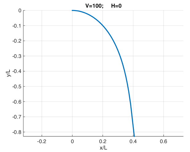
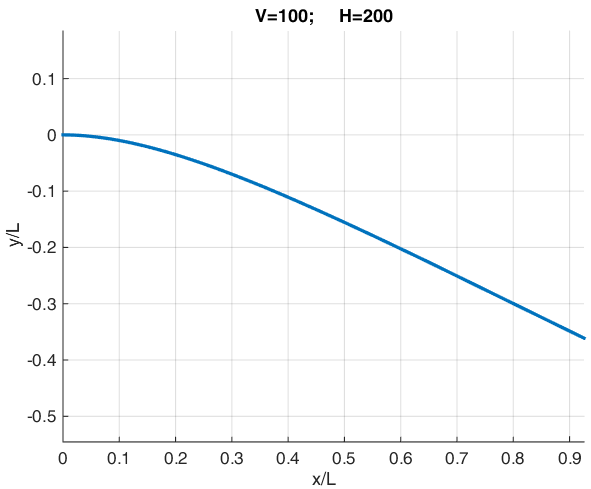
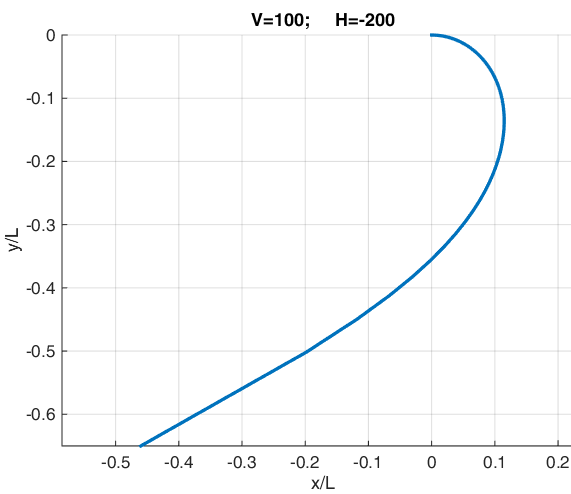
Figure 2. Deformed centerlines for the three fixed-direction end-force combinations.

For $V=100\ \mathrm{N}$ and $H=-200\ \mathrm{N}$ , both tested MATLAB versions returned:

Quantity	Value
Elliptic parameter	$m=0.999682400374605$
Loaded-end coordinate	$x_A=-46.0156\ \mathrm{mm}$
Loaded-end coordinate	$y_A=-65.0130\ \mathrm{mm}$
Maximum bending-moment magnitude	$\max\|M\|=8401.05\ \mathrm{N\,mm}$

Independent bending-moment check

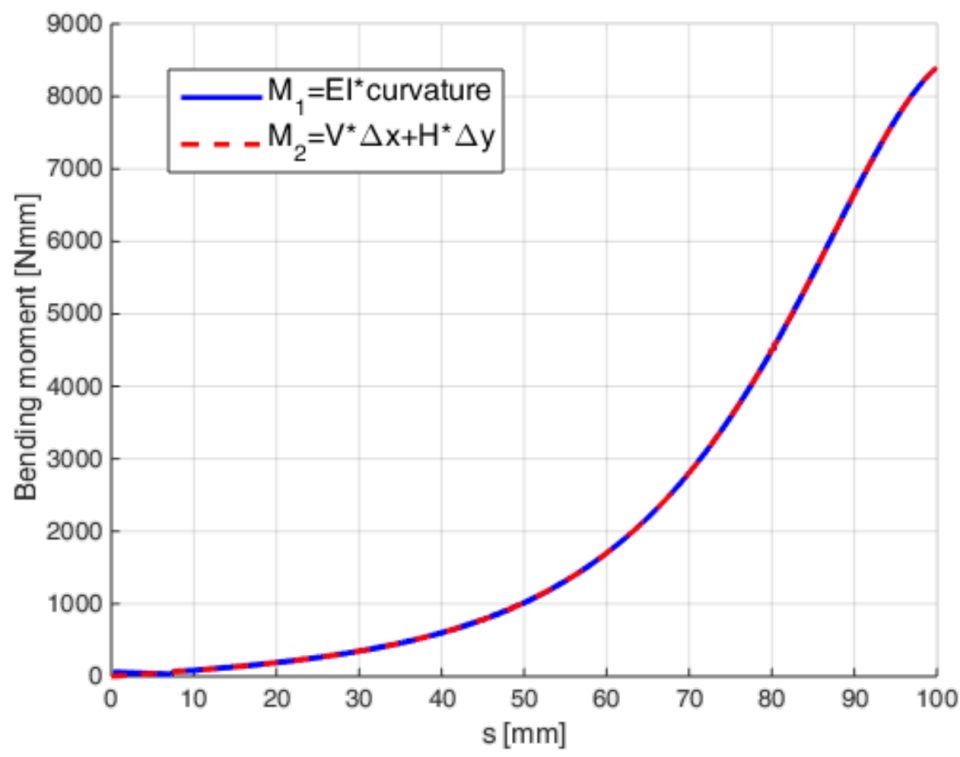
The bending moment is evaluated in two independent ways. The first uses the centerline curvature:

M_1=EI\kappa,\qquad \kappa=\frac{d\varphi}{ds}

The second follows from equilibrium of the end-force components, with $(x_A,y_A)$ at the loaded end:

M_2=-V(x-x_A)-H(y-y_A)

A consistent solution must satisfy

M_1=M_2

Comparison of the bending moment from curvature and from end-force equilibrium — Figure 3.Moment comparison for $V=100\ \mathrm{N}$ and $H=-200\ \mathrm{N}$ . The two curves are visually indistinguishable at the plotted scale.

Program files

The archive contains three commented MATLAB files and a README describing the model, the required toolbox, and the input convention.

MCantilever elastica MATLAB package3 MATLAB files + README · tested in R2017b and R2026aDownload ZIP

References

S. P. Timoshenko and J. M. Gere, Theory of Elastic Stability, 2nd ed., McGraw–Hill, New York, 1961.
F. De Bona and S. Zelenika, “A generalized elastica-type approach to the analysis of large displacements of spring-strips”, Proceedings of the Institution of Mechanical Engineers, Part C: Journal of Mechanical Engineering Science, vol. 211, no. 7, pp. 509–517, 1997.
MathWorks, MATLAB documentation for ellipticF, ellipticK, and ellipticE