Large Displacements of a Cantilever Beam — Finite-Difference Method

Model and assumptions

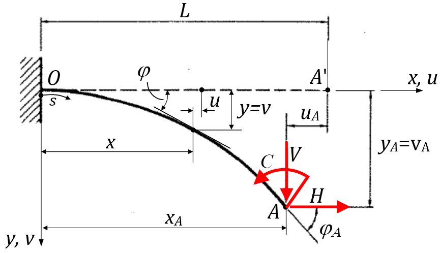
Consider a straight cantilever beam of length $L$ , constant cross-section, and linear elastic material. The free end is subjected to the force components $H$ and $V$ , and to an end couple $C$ .

MaterialLinear elastic

StrainSmall

DisplacementPotentially large

The Euler–Bernoulli model is used. The neutral axis is treated as inextensible and the rotation $\varphi$ is the slope of the deformed neutral axis. For this finite-difference formulation, $x$ is positive to the right and $y$ is positive downward, exactly as defined in Figure 1 and in the program.

Cantilever geometry with deformed neutral axis, arc-length coordinate, free-end forces, couple, and displacement components — Figure 1. Geometry, signs, and notation for the cantilever beam.

$E$: Young's modulus
$I$: Geometrical moment of inertia of the cross-section
$M$: Bending moment
$\kappa$: Curvature
$s$: Arc-length coordinate along the neutral axis

Beam equilibrium

At an arbitrary point of the deformed beam, the bending moment follows from equilibrium of the free-end loads:

EI\kappa=M=C+V\left(x_A-x\right)-H\left(y_A-y\right)

The exact kinematic relations for the inextensible centerline are:

\kappa=\frac{d\varphi}{ds},\qquad \frac{dx}{ds}=\cos\varphi,\qquad \frac{dy}{ds}=\sin\varphi

The boundary condition at the clamped end $O$ is $\varphi(0)=0$ . The free-end coordinates $x_A$ and $y_A$ are part of the nonlinear solution.

Finite-difference equations

Divide the beam into $n-1$ equal intervals of length $h=L/(n-1)$ . Node 1 is at the clamp and node $n$ is at the free end. Writing the equilibrium equation at the midpoint between nodes $i-1$ and $i$ gives:

\frac{EI}{h}\left(\varphi_i-\varphi_{i-1}\right)=C+V\left(x_A-\frac{x_i+x_{i-1}}{2}\right)-H\left(y_A-\frac{y_i+y_{i-1}}{2}\right),\qquad i=2,\ldots,n

With $\varphi_1=0$ , the first residual equation is:

\Psi_1=\frac{EI}{h}\varphi_2+C-V\left(x_n-\frac{x_2}{2}\right)+H\left(y_n-\frac{y_2}{2}\right)=0

Subtracting adjacent midpoint equations eliminates the free-end coordinates from the remaining equations. For $i=2,\ldots,n-1$ ,

\begin{aligned}\Psi_i={}&\frac{EI}{h}\left(\varphi_{i+1}-2\varphi_i+\varphi_{i-1}\right)\\&+\frac{Vh}{2}\left[\cos\frac{\varphi_i+\varphi_{i+1}}{2}+\cos\frac{\varphi_{i-1}+\varphi_i}{2}\right]\\&-\frac{Hh}{2}\left[\sin\frac{\varphi_i+\varphi_{i+1}}{2}+\sin\frac{\varphi_{i-1}+\varphi_i}{2}\right]=0\end{aligned}

The centerline is reconstructed after each update from the midpoint rotations:

x_i=x_{i-1}+h\cos\frac{\varphi_i+\varphi_{i-1}}{2},\qquad y_i=y_{i-1}+h\sin\frac{\varphi_i+\varphi_{i-1}}{2}

Modified Newton iteration

The residual vector has $n-1$ components. Its local equations use the exact derivatives shown by the program. In the first tangent equation, however, the current values of $x_n$ and $y_n$ are held fixed. The method is therefore a modified Newton iteration, not a full Newton method.

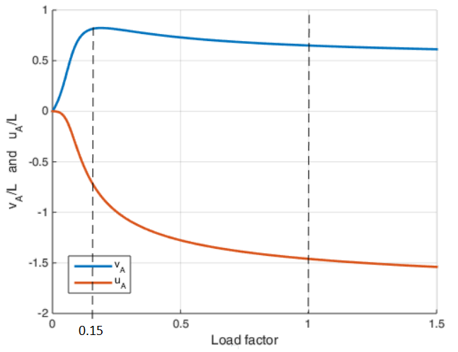
\boldsymbol{J}\,\Delta\boldsymbol{\varphi}=\boldsymbol{\Psi},\qquad \boldsymbol{\varphi}^{(j+1)}=\boldsymbol{\varphi}^{(j)}-\gamma\,\Delta\boldsymbol{\varphi}

For the strongly nonlinear example below, the program uses $\gamma=0.025$ . This small relaxation factor makes the modified iteration robust when the free-end displacement is already large. For load factors below about $0.15$ , the program can use $\gamma=1$ and convergence is much faster.

Jacobian convention

The first row is intentionally approximate because it freezes the current free-end coordinates. The remaining rows are differentiated exactly. This is the iteration implemented and verified here.

MATLAB implementation

The program is a single commented MATLAB script. It defines the beam, assembles the residual and tangent matrix, applies the under-relaxed rotation correction, and reconstructs the deformed centerline.

cantilever.mModified Newton update

% Under-relaxed correction of the nodal rotations.
df = J\psi;
df = [0; df];
f = f - sr*df;
err = sqrt(df'*df/(2*n));

% Reconstruct the centerline from midpoint rotations.
fm = (f(2:n)+f(1:n-1))/2;
x = [0; cumsum(cos(fm)*h)];
y = [0; cumsum(sin(fm)*h)];

MATLAB compatibility

Tested in MATLAB R2017b and MATLAB R2026a. The code uses standard MATLAB syntax and is expected to be compatible with intermediate and newer MATLAB versions. It uses only core MATLAB functions and does not require an additional toolbox.

Numerical examples

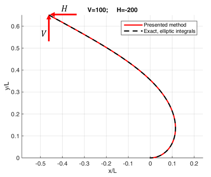
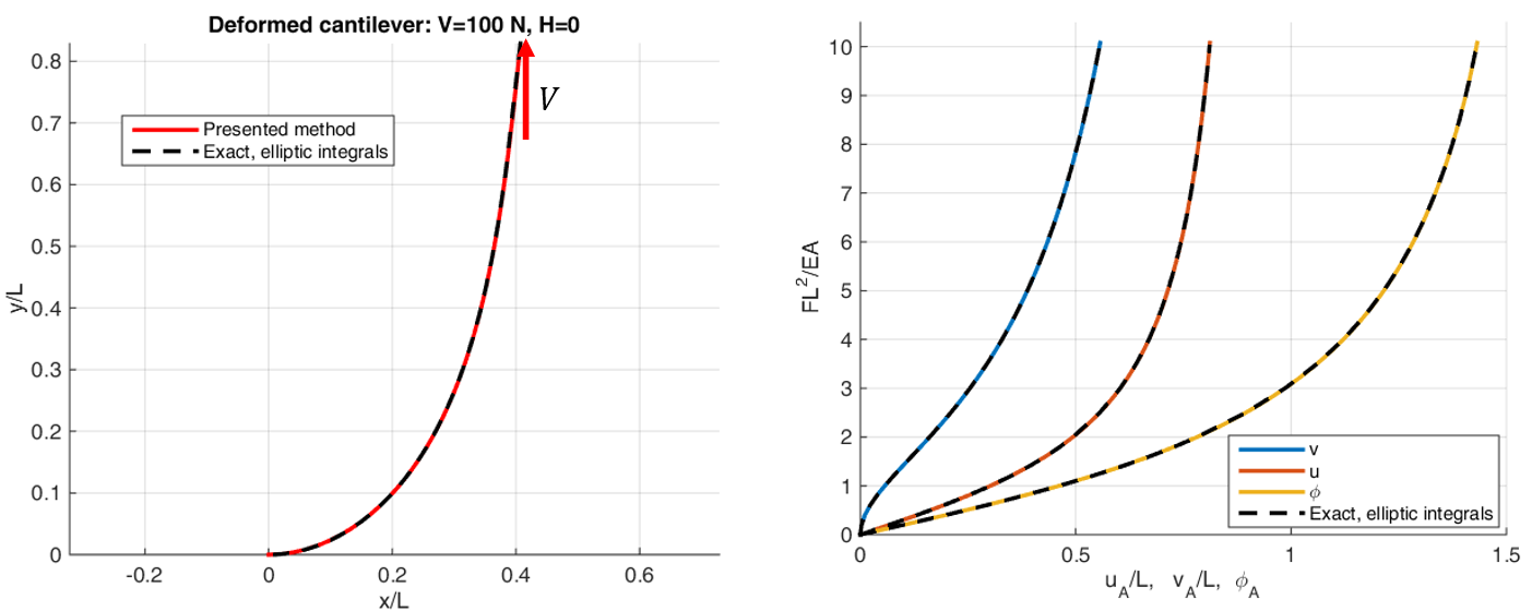
The beam has $L=100\ \mathrm{mm}$ , a rectangular cross-section $5\times1\ \mathrm{mm}$ (width × thickness), and $E=2\times10^5\ \mathrm{MPa}$ .

Deformed cantilever for vertical load 100 newtons and horizontal load minus 200 newtons, compared with the exact elastica — Figure 2. Deformed cantilever for V = 100 N and H = −200 N. The solid curve is the finite-difference solution and the dashed curve is the exact elastica solution.

Normalized free-end horizontal and vertical displacements as functions of load factor for vertical load 100 newtons and horizontal load minus 200 newtons — Figure 3. Normalized free-end displacements versus load factor for V = 100 N and H = −200 N.

Two-panel comparison with the exact elastica for vertical load 100 newtons and zero horizontal load — Figure 4. Comparison with the exact elastica for V = 100 N and H = 0. Left: deformed cantilever under maximum force. Right: load factor versus normalized free-end displacements and free-end rotation. Solid curves are obtained by the finite-difference method; dashed curves are the exact solution [1].

Program files

The archive contains the commented solver, a numerical Jacobian-check script, and a README describing the sign convention and iteration method.

MCantilever finite-difference MATLAB package2 MATLAB files + README · tested in R2017b and R2026aDownload ZIP

References

K. Mattiasson, “Numerical results from large deflection beam and frame problems analysed by means of elliptic integrals,” International Journal for Numerical Methods in Engineering, vol. 16, pp. 145–153, 1981.