Section 22.1 of Chapter 22: Large displacements cantilever beam

Curvature tensor of a 3D slender beam. Euler–Bernoulli beam theory

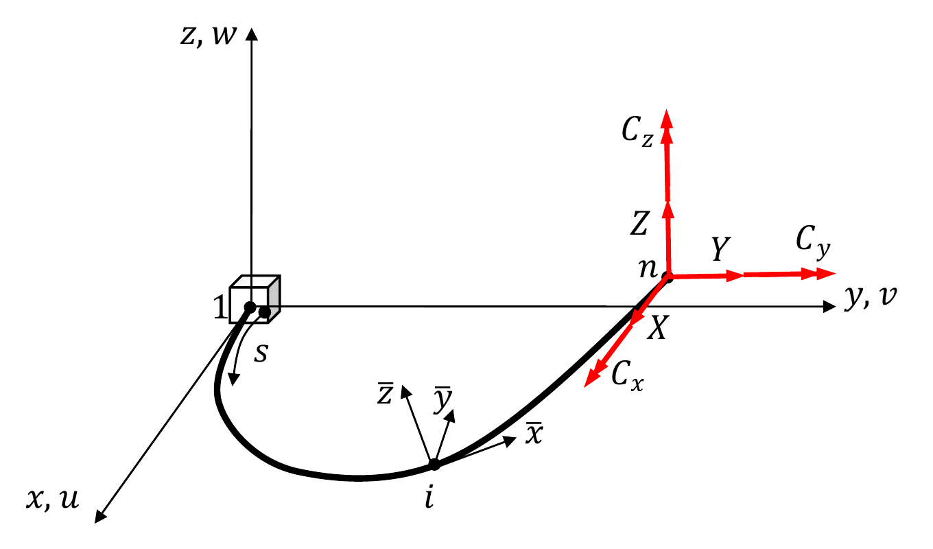
The figure below depicts a deformed 3D slender beam. The local reference frame (xˉ,yˉ,zˉ)(\bar x,\bar y,\bar z) is defined as follows: the xˉ\bar x-axis is tangent to the deformed beam axis, while the yˉ\bar y- and zˉ\bar z-axes coincide with the principal centroidal axes of the beam cross-section. The reference frame (x,y,z)(x,y,z) is the global reference frame.

Deformed 3D slender beam with global axes and local cross-section axes

The orientation of the local reference frame is defined by the rotation matrix R\boldsymbol{R}. In this section, R\boldsymbol{R} is used as a passive transformation matrix from the global reference frame to the local reference frame. Thus, for any vector,

vˉ=Rv,v=RTvˉ.\bar{\boldsymbol{v}}=\boldsymbol{R}\,\boldsymbol{v},\qquad\boldsymbol{v}=\boldsymbol{R}^T\bar{\boldsymbol{v}}.

Here xˉ\bar x denotes the local beam-axis coordinate, defined along the locus of the cross-section centroids. For a general curved beam, an arc-length coordinate ss could also be used; here xˉ\bar x is preferred because the formulation will later be specialized to straight beams with small deformations.

Let us consider two very close cross-sections located at a distance dxˉd\bar x. The first one is characterized by the rotation matrix R\boldsymbol{R}. The second cross-section is rotated with respect to the first one by the infinitesimal angles dφxˉd\varphi_{\bar x}, dφyˉd\varphi_{\bar y}, and dφzˉd\varphi_{\bar z} about the xˉ\bar x-, yˉ\bar y-, and zˉ\bar z-axes of the local reference frame, respectively.

The corresponding infinitesimal relative rotation matrix, expressed in the local reference frame of the first cross-section, is

R0=[1dφzˉdφyˉdφzˉ1dφxˉdφyˉdφxˉ1].\boldsymbol{R}_0=\begin{bmatrix}1&-d\varphi_{\bar z}&d\varphi_{\bar y}\\d\varphi_{\bar z}&1&-d\varphi_{\bar x}\\-d\varphi_{\bar y}&d\varphi_{\bar x}&1\end{bmatrix}.

Consequently, the rotation matrix of the second cross-section is

R2=R0R.\boldsymbol{R}_2=\boldsymbol{R}_0\boldsymbol{R}.

Therefore,

dR=R2R=(R0I)R=[0dφzˉdφyˉdφzˉ0dφxˉdφyˉdφxˉ0]R.d\boldsymbol{R}=\boldsymbol{R}_2-\boldsymbol{R}=(\boldsymbol{R}_0-\boldsymbol{I})\boldsymbol{R}=\begin{bmatrix}0&-d\varphi_{\bar z}&d\varphi_{\bar y}\\d\varphi_{\bar z}&0&-d\varphi_{\bar x}\\-d\varphi_{\bar y}&d\varphi_{\bar x}&0\end{bmatrix}\boldsymbol{R}.

Dividing by dxˉd\bar x,

dRdxˉ=[0dφzˉdxˉdφyˉdxˉdφzˉdxˉ0dφxˉdxˉdφyˉdxˉdφxˉdxˉ0]R.\frac{d\boldsymbol{R}}{d\bar x}=\begin{bmatrix}0&-\dfrac{d\varphi_{\bar z}}{d\bar x}&\dfrac{d\varphi_{\bar y}}{d\bar x}\\[4pt]\dfrac{d\varphi_{\bar z}}{d\bar x}&0&-\dfrac{d\varphi_{\bar x}}{d\bar x}\\[4pt]-\dfrac{d\varphi_{\bar y}}{d\bar x}&\dfrac{d\varphi_{\bar x}}{d\bar x}&0\end{bmatrix}\boldsymbol{R}.

We define the curvature components:

κxˉ=dφxˉdxˉ,κyˉ=dφyˉdxˉ,κzˉ=dφzˉdxˉ.\kappa_{\bar x}=\frac{d\varphi_{\bar x}}{d\bar x},\qquad\kappa_{\bar y}=\frac{d\varphi_{\bar y}}{d\bar x},\qquad\kappa_{\bar z}=\frac{d\varphi_{\bar z}}{d\bar x}.

The curvature tensor is

κ~=[0κzˉκyˉκzˉ0κxˉκyˉκxˉ0],\widetilde{\boldsymbol{\kappa}}=\begin{bmatrix}0&-\kappa_{\bar z}&\kappa_{\bar y}\\\kappa_{\bar z}&0&-\kappa_{\bar x}\\-\kappa_{\bar y}&\kappa_{\bar x}&0\end{bmatrix},

and

dRdxˉ=κ~Rorκ~=dRdxˉRT.\boxed{\frac{d\boldsymbol{R}}{d\bar x}=\widetilde{\boldsymbol{\kappa}}\boldsymbol{R}}\qquad\text{or}\qquad\boxed{\widetilde{\boldsymbol{\kappa}}=\frac{d\boldsymbol{R}}{d\bar x}\boldsymbol{R}^T}.

The curvature tensor is skew-symmetric:

κ~T=κ~.\widetilde{\boldsymbol{\kappa}}^{\,T}=-\widetilde{\boldsymbol{\kappa}}.

The curvature components can also be organized as a vector:

κ={κxˉκyˉκzˉ}.\boldsymbol{\kappa}=\begin{Bmatrix}\kappa_{\bar x}\\\kappa_{\bar y}\\\kappa_{\bar z}\end{Bmatrix}.

The components κxˉ,κyˉ,κzˉ\kappa_{\bar x},\kappa_{\bar y},\kappa_{\bar z} are not the curvatures of the beam axis in the usual differential-geometric sense. They are defined from the relative infinitesimal rotation of two neighbouring cross-sections per unit length about the local axes. Thus, κxˉdxˉ\kappa_{\bar x}\,d\bar x is the relative infinitesimal rotation about the local xˉ\bar x-axis, κyˉdxˉ\kappa_{\bar y}\,d\bar x is the relative infinitesimal rotation about the local yˉ\bar y-axis, and κzˉdxˉ\kappa_{\bar z}\,d\bar x is the relative infinitesimal rotation about the local zˉ\bar z-axis.

According to the sign convention adopted in the Nomenclature, the corresponding constitutive relations are

Mxˉ=GJκxˉ,Myˉ=EIyˉκyˉ,Mzˉ=EIzˉκzˉ,M_{\bar x}=GJ\,\kappa_{\bar x},\qquad M_{\bar y}=-EI_{\bar y}\,\kappa_{\bar y},\qquad M_{\bar z}=EI_{\bar z}\,\kappa_{\bar z},

see Section 22.2.

It is also easy to prove directly that κ~\widetilde{\boldsymbol{\kappa}} is skew-symmetric [1]. Since R\boldsymbol{R} is an orthogonal matrix,

RRT=I.\boldsymbol{R}\boldsymbol{R}^T=\boldsymbol{I}.

Differentiating with respect to xˉ\bar x,

dRdxˉRT+RdRTdxˉ=0.\frac{d\boldsymbol{R}}{d\bar x}\boldsymbol{R}^T+\boldsymbol{R}\frac{d\boldsymbol{R}^T}{d\bar x}=\boldsymbol{0}.

Hence,

(dRdxˉRT)T=RdRTdxˉ=dRdxˉRT,\left(\frac{d\boldsymbol{R}}{d\bar x}\boldsymbol{R}^T\right)^T=\boldsymbol{R}\frac{d\boldsymbol{R}^T}{d\bar x}=-\frac{d\boldsymbol{R}}{d\bar x}\boldsymbol{R}^T,

and therefore

κ~T=κ~.\widetilde{\boldsymbol{\kappa}}^{\,T}=-\widetilde{\boldsymbol{\kappa}}.

References

1. Da Lozzo, E. C., Geometrically exact three-dimensional beam theory: modeling and FEM implementation for statics and dynamics analysis, Università degli Studi di Pavia, 2010.