A simple numerical method to study a 3D cantilever with large displacements, utilising finite differences, is shown in this section. It is similar to that presented in Chapter 4 for the 2D case.
Geometry Straight slender beam, constant cross-section
Strain Small
Material Linear
Displacement Large
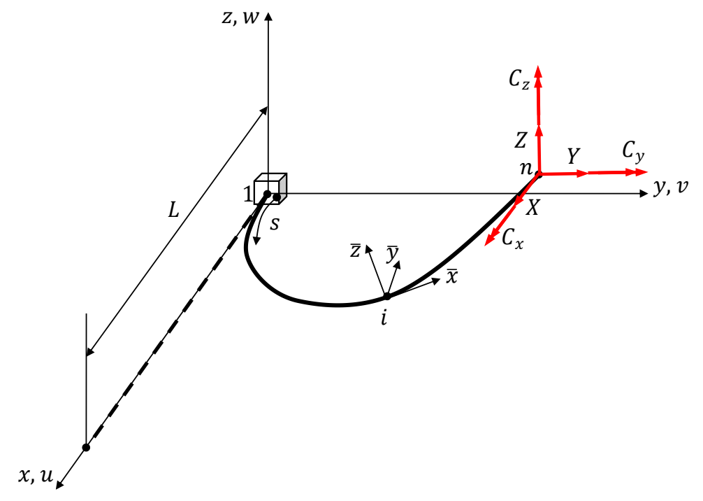
Figure 1. Initially straight cantilever and deformed beam with applied end forces and moments.Initially, a straight beam lies on the x x x
Euler–Bernoulli beam model (i.e. the effect of the shear force is neglected) for an initially curved beam:
D ( κ − κ 0 ) = M ‾ (*)
\boldsymbol{D}(\boldsymbol{\kappa}-\boldsymbol{\kappa}_0)
=
\overline{\boldsymbol{M}}
\tag{*}
D ( κ − κ 0 ) = M ( * ) or:
{ G I t ( κ x ˉ − κ 0 x ˉ ) = M x ˉ , E I y ˉ ( κ y ˉ − κ 0 y ˉ ) = M y ˉ , E I z ˉ ( κ z ˉ − κ 0 z ˉ ) = M z ˉ .
\left\{
\begin{array}{l}
GI_t(\kappa_{\bar x}-\kappa_{0\bar x})=M_{\bar x},\\[2mm]
EI_{\bar y}(\kappa_{\bar y}-\kappa_{0\bar y})=M_{\bar y},\\[2mm]
EI_{\bar z}(\kappa_{\bar z}-\kappa_{0\bar z})=M_{\bar z}.
\end{array}
\right.
⎩ ⎨ ⎧ G I t ( κ x ˉ − κ 0 x ˉ ) = M x ˉ , E I y ˉ ( κ y ˉ − κ 0 y ˉ ) = M y ˉ , E I z ˉ ( κ z ˉ − κ 0 z ˉ ) = M z ˉ . E E E I t , I y ˉ , I z ˉ I_t,I_{\bar y},I_{\bar z} I t , I y ˉ , I z ˉ M x ˉ , M y ˉ , M z ˉ M_{\bar x},M_{\bar y},M_{\bar z} M x ˉ , M y ˉ , M z ˉ The above equations are written in the local reference frame ( x ˉ , y ˉ , z ˉ ) (\bar x,\bar y,\bar z) ( x ˉ , y ˉ , z ˉ ) x ˉ \bar x x ˉ y ˉ , z ˉ \bar y,\bar z y ˉ , z ˉ
D = [ G I t 0 0 0 E I y ˉ 0 0 0 E I z ˉ ] , κ = { κ x ˉ κ y ˉ κ z ˉ } ,
\boldsymbol{D}=
\begin{bmatrix}
GI_t&0&0\\
0&EI_{\bar y}&0\\
0&0&EI_{\bar z}
\end{bmatrix},
\qquad
\boldsymbol{\kappa}=
\left\{
\begin{array}{c}
\kappa_{\bar x}\\
\kappa_{\bar y}\\
\kappa_{\bar z}
\end{array}
\right\},
D = G I t 0 0 0 E I y ˉ 0 0 0 E I z ˉ , κ = ⎩ ⎨ ⎧ κ x ˉ κ y ˉ κ z ˉ ⎭ ⎬ ⎫ , κ 0 = { κ 0 x ˉ κ 0 y ˉ κ 0 z ˉ } , M ‾ = { M x ˉ M y ˉ M z ˉ } .
\boldsymbol{\kappa}_0=
\left\{
\begin{array}{c}
\kappa_{0\bar x}\\
\kappa_{0\bar y}\\
\kappa_{0\bar z}
\end{array}
\right\},
\qquad
\overline{\boldsymbol{M}}=
\left\{
\begin{array}{c}
M_{\bar x}\\
M_{\bar y}\\
M_{\bar z}
\end{array}
\right\}.
κ 0 = ⎩ ⎨ ⎧ κ 0 x ˉ κ 0 y ˉ κ 0 z ˉ ⎭ ⎬ ⎫ , M = ⎩ ⎨ ⎧ M x ˉ M y ˉ M z ˉ ⎭ ⎬ ⎫ . To preserve both the geometrical definition of the curvature vector and the moment sign convention adopted in the Nomenclature, we introduce the sign matrix:
S = [ 1 0 0 0 − 1 0 0 0 1 ] .
\boldsymbol{S}=
\begin{bmatrix}
1&0&0\\
0&-1&0\\
0&0&1
\end{bmatrix}.
S = 1 0 0 0 − 1 0 0 0 1 . The local moment vector according to the Nomenclature, distinguished by the superscript N N N
M ‾ N = S M ‾ ,
\overline{\boldsymbol{M}}^{\,N}=\boldsymbol{S}\,\overline{\boldsymbol{M}},
M N = S M , or explicitly,
M x ˉ = G I t ( κ x ˉ − κ 0 x ˉ ) , M y ˉ N = − E I y ˉ ( κ y ˉ − κ 0 y ˉ ) , M z ˉ = E I z ˉ ( κ z ˉ − κ 0 z ˉ ) .
M_{\bar x}=GI_t(\kappa_{\bar x}-\kappa_{0\bar x}),\qquad
M_{\bar y}^{N}=-EI_{\bar y}(\kappa_{\bar y}-\kappa_{0\bar y}),\qquad
M_{\bar z}=EI_{\bar z}(\kappa_{\bar z}-\kappa_{0\bar z}).
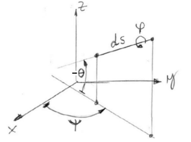
M x ˉ = G I t ( κ x ˉ − κ 0 x ˉ ) , M y ˉ N = − E I y ˉ ( κ y ˉ − κ 0 y ˉ ) , M z ˉ = E I z ˉ ( κ z ˉ − κ 0 z ˉ ) . The position of a beam arc d s ds d s x ˉ \bar x x ˉ Section 21.2 .
Figure 2. Tait–Bryan angles defining the beam arc.We assume that the local reference frame is obtained as follows: initially the local frame coincides with the global one and we apply three consecutive rotations in this order, called z y ′ x ′ ′ zy'x'' z y ′ x ′′
a rotation of angle ψ \psi ψ z z z a rotation of angle θ \theta θ y y y y ′ y' y ′ finally, a rotation of angle φ \varphi φ x x x x ′ ′ x'' x ′′ The rotation matrix is, see Section 21.2 :
R = [ cos ψ cos θ sin ψ cos θ − sin θ − sin ψ cos φ + cos ψ sin θ sin φ cos ψ cos φ + sin ψ sin θ sin φ cos θ sin φ sin ψ sin φ + cos ψ sin θ cos φ − cos ψ sin φ + sin ψ sin θ cos φ cos θ cos φ ] .
\boldsymbol{R}=
\begin{bmatrix}
\cos\psi\cos\theta&
\sin\psi\cos\theta&
-\sin\theta\\
-\sin\psi\cos\varphi+\cos\psi\sin\theta\sin\varphi&
\cos\psi\cos\varphi+\sin\psi\sin\theta\sin\varphi&
\cos\theta\sin\varphi\\
\sin\psi\sin\varphi+\cos\psi\sin\theta\cos\varphi&
-\cos\psi\sin\varphi+\sin\psi\sin\theta\cos\varphi&
\cos\theta\cos\varphi
\end{bmatrix}.
R = cos ψ cos θ − sin ψ cos φ + cos ψ sin θ sin φ sin ψ sin φ + cos ψ sin θ cos φ sin ψ cos θ cos ψ cos φ + sin ψ sin θ sin φ − cos ψ sin φ + sin ψ sin θ cos φ − sin θ cos θ sin φ cos θ cos φ . As in Section 22.1 , R \boldsymbol{R} R
v ‾ = R v , v = R T v ‾ .
\overline{\boldsymbol{v}}=\boldsymbol{R}\,\boldsymbol{v},
\qquad
\boldsymbol{v}=\boldsymbol{R}^T\overline{\boldsymbol{v}}.
v = R v , v = R T v . According to Section 22.1 , the curvature tensor is defined by [1] :
κ ~ = d R d x ˉ R T ,
\widetilde{\boldsymbol{\kappa}}
=
\frac{d\boldsymbol{R}}{d\bar x}\boldsymbol{R}^T,
κ = d x ˉ d R R T , where
κ ~ = [ 0 − κ z ˉ κ y ˉ κ z ˉ 0 − κ x ˉ − κ y ˉ κ x ˉ 0 ] .
\widetilde{\boldsymbol{\kappa}}
=
\begin{bmatrix}
0&-\kappa_{\bar z}&\kappa_{\bar y}\\
\kappa_{\bar z}&0&-\kappa_{\bar x}\\
-\kappa_{\bar y}&\kappa_{\bar x}&0
\end{bmatrix}.
κ = 0 κ z ˉ − κ y ˉ − κ z ˉ 0 κ x ˉ κ y ˉ − κ x ˉ 0 . Using the Tait–Bryan parametrization, the curvature vector results [2] :
{ κ x ˉ κ y ˉ κ z ˉ } = [ − sin θ 0 1 cos θ sin φ cos φ 0 cos θ cos φ − sin φ 0 ] { ψ ′ θ ′ φ ′ } ,
\left\{
\begin{array}{c}
\kappa_{\bar x}\\
\kappa_{\bar y}\\
\kappa_{\bar z}
\end{array}
\right\}
=
\begin{bmatrix}
-\sin\theta&0&1\\
\cos\theta\sin\varphi&\cos\varphi&0\\
\cos\theta\cos\varphi&-\sin\varphi&0
\end{bmatrix}
\left\{
\begin{array}{c}
\psi'\\
\theta'\\
\varphi'
\end{array}
\right\},
⎩ ⎨ ⎧ κ x ˉ κ y ˉ κ z ˉ ⎭ ⎬ ⎫ = − sin θ cos θ sin φ cos θ cos φ 0 cos φ − sin φ 1 0 0 ⎩ ⎨ ⎧ ψ ′ θ ′ φ ′ ⎭ ⎬ ⎫ , or
κ = A α ′ ,
\boldsymbol{\kappa}
=
\boldsymbol{A}\,\boldsymbol{\alpha}',
κ = A α ′ , where
A = [ − sin θ 0 1 cos θ sin φ cos φ 0 cos θ cos φ − sin φ 0 ] ,
\boldsymbol{A}=
\begin{bmatrix}
-\sin\theta&0&1\\
\cos\theta\sin\varphi&\cos\varphi&0\\
\cos\theta\cos\varphi&-\sin\varphi&0
\end{bmatrix},
A = − sin θ cos θ sin φ cos θ cos φ 0 cos φ − sin φ 1 0 0 , α ′ = { ψ ′ θ ′ φ ′ } , ψ ′ = d ψ d s , θ ′ = d θ d s , φ ′ = d φ d s .
\boldsymbol{\alpha}'=
\left\{
\begin{array}{c}
\psi'\\
\theta'\\
\varphi'
\end{array}
\right\},
\qquad
\psi'=\frac{d\psi}{ds},
\qquad
\theta'=\frac{d\theta}{ds},
\qquad
\varphi'=\frac{d\varphi}{ds}.
α ′ = ⎩ ⎨ ⎧ ψ ′ θ ′ φ ′ ⎭ ⎬ ⎫ , ψ ′ = d s d ψ , θ ′ = d s d θ , φ ′ = d s d φ . In this section, we will analyse only an initially straight flexible beam:
κ 0 = 0 3 × 1 .
\boldsymbol{\kappa}_0=\boldsymbol{0}_{3\times1}.
κ 0 = 0 3 × 1 . At each point ( x , y , z ) (x,y,z) ( x , y , z )
D κ = M ‾ ,
\boldsymbol{D}\boldsymbol{\kappa}
=
\overline{\boldsymbol{M}},
D κ = M , or
D A α ′ = M ‾ .
\boxed{
\boldsymbol{D}\boldsymbol{A}\,\boldsymbol{\alpha}'
=
\overline{\boldsymbol{M}}.
}
D A α ′ = M . The moment in the current cross-section ( x , y , z ) (x,y,z) ( x , y , z )
M = { x n − x y n − y z n − z } × { X Y Z } + { C x C y C z } ,
\boldsymbol{M}=
\left\{
\begin{array}{c}
x_n-x\\
y_n-y\\
z_n-z
\end{array}
\right\}
\times
\left\{
\begin{array}{c}
X\\
Y\\
Z
\end{array}
\right\}
+
\left\{
\begin{array}{c}
C_x\\
C_y\\
C_z
\end{array}
\right\},
M = ⎩ ⎨ ⎧ x n − x y n − y z n − z ⎭ ⎬ ⎫ × ⎩ ⎨ ⎧ X Y Z ⎭ ⎬ ⎫ + ⎩ ⎨ ⎧ C x C y C z ⎭ ⎬ ⎫ , or
M = { Z ( y n − y ) − Y ( z n − z ) + C x X ( z n − z ) − Z ( x n − x ) + C y Y ( x n − x ) − X ( y n − y ) + C z } ,
\boldsymbol{M}=
\left\{
\begin{array}{c}
Z(y_n-y)-Y(z_n-z)+C_x\\
X(z_n-z)-Z(x_n-x)+C_y\\
Y(x_n-x)-X(y_n-y)+C_z
\end{array}
\right\},
M = ⎩ ⎨ ⎧ Z ( y n − y ) − Y ( z n − z ) + C x X ( z n − z ) − Z ( x n − x ) + C y Y ( x n − x ) − X ( y n − y ) + C z ⎭ ⎬ ⎫ , where × \times ×
The moments in the local reference frame are
M ‾ = R M .
\boxed{
\overline{\boldsymbol{M}}
=
\boldsymbol{R}\,\boldsymbol{M}.
}
M = R M . The beam is divided into n − 1 n-1 n − 1 n n n
h = L n − 1 ,
h=\frac{L}{n-1},
h = n − 1 L , where L L L
With finite differences, the differential equation
D A α ′ = M ‾
\boldsymbol{D}\boldsymbol{A}\,\boldsymbol{\alpha}'
=
\overline{\boldsymbol{M}}
D A α ′ = M becomes, using backward differences,
D A i { ψ i − ψ i − 1 h θ i − θ i − 1 h φ i − φ i − 1 h } = R i { Z ( y n − y i ) − Y ( z n − z i ) + C x X ( z n − z i ) − Z ( x n − x i ) + C y Y ( x n − x i ) − X ( y n − y i ) + C z } , i = 2 , … , n .
\boldsymbol{D}\boldsymbol{A}_i
\left\{
\begin{array}{c}
\dfrac{\psi_i-\psi_{i-1}}{h}\\[3mm]
\dfrac{\theta_i-\theta_{i-1}}{h}\\[3mm]
\dfrac{\varphi_i-\varphi_{i-1}}{h}
\end{array}
\right\}
=
\boldsymbol{R}_i
\left\{
\begin{array}{c}
Z(y_n-y_i)-Y(z_n-z_i)+C_x\\
X(z_n-z_i)-Z(x_n-x_i)+C_y\\
Y(x_n-x_i)-X(y_n-y_i)+C_z
\end{array}
\right\},
\qquad i=2,\ldots,n.
D A i ⎩ ⎨ ⎧ h ψ i − ψ i − 1 h θ i − θ i − 1 h φ i − φ i − 1 ⎭ ⎬ ⎫ = R i ⎩ ⎨ ⎧ Z ( y n − y i ) − Y ( z n − z i ) + C x X ( z n − z i ) − Z ( x n − x i ) + C y Y ( x n − x i ) − X ( y n − y i ) + C z ⎭ ⎬ ⎫ , i = 2 , … , n . The condition at the clamped end, node 1, is
ψ 1 = 0 , θ 1 = 0 , φ 1 = 0.
\psi_1=0,\qquad
\theta_1=0,\qquad
\varphi_1=0.
ψ 1 = 0 , θ 1 = 0 , φ 1 = 0. R i \boldsymbol{R}_i R i i i i ψ i , θ i , φ i \psi_i,\theta_i,\varphi_i ψ i , θ i , φ i The above equation can be rewritten in a recursive manner, making it very easy to program:
{ ψ i θ i φ i } = h [ D A i ] − 1 R i { Z ( y n − y i ) − Y ( z n − z i ) + C x X ( z n − z i ) − Z ( x n − x i ) + C y Y ( x n − x i ) − X ( y n − y i ) + C z } + { ψ i − 1 θ i − 1 φ i − 1 } , i = 2 , … , n .
\left\{
\begin{array}{c}
\psi_i\\
\theta_i\\
\varphi_i
\end{array}
\right\}
=
h[\boldsymbol{D}\boldsymbol{A}_i]^{-1}\boldsymbol{R}_i
\left\{
\begin{array}{c}
Z(y_n-y_i)-Y(z_n-z_i)+C_x\\
X(z_n-z_i)-Z(x_n-x_i)+C_y\\
Y(x_n-x_i)-X(y_n-y_i)+C_z
\end{array}
\right\}
+
\left\{
\begin{array}{c}
\psi_{i-1}\\
\theta_{i-1}\\
\varphi_{i-1}
\end{array}
\right\},
\qquad i=2,\ldots,n.
⎩ ⎨ ⎧ ψ i θ i φ i ⎭ ⎬ ⎫ = h [ D A i ] − 1 R i ⎩ ⎨ ⎧ Z ( y n − y i ) − Y ( z n − z i ) + C x X ( z n − z i ) − Z ( x n − x i ) + C y Y ( x n − x i ) − X ( y n − y i ) + C z ⎭ ⎬ ⎫ + ⎩ ⎨ ⎧ ψ i − 1 θ i − 1 φ i − 1 ⎭ ⎬ ⎫ , i = 2 , … , n . Several iterations are needed: using the above recursive equation, at the j j j
α i = { ψ i θ i φ i } , i = 1 , … , n ,
\boldsymbol{\alpha}_i=
\left\{
\begin{array}{c}
\psi_i\\
\theta_i\\
\varphi_i
\end{array}
\right\},
\qquad i=1,\ldots,n,
α i = ⎩ ⎨ ⎧ ψ i θ i φ i ⎭ ⎬ ⎫ , i = 1 , … , n , are found as functions of the nodal coordinates obtained in the previous iteration j − 1 j-1 j − 1
The Cartesian coordinates of a point located at the curvilinear coordinate s s s
{ x ( s ) y ( s ) z ( s ) } = ∫ 0 s { cos ψ cos θ sin ψ cos θ − sin θ } d s ,
\left\{
\begin{array}{c}
x(s)\\
y(s)\\
z(s)
\end{array}
\right\}
=
\int_0^s
\left\{
\begin{array}{c}
\cos\psi\cos\theta\\
\sin\psi\cos\theta\\
-\sin\theta
\end{array}
\right\}\,ds,
⎩ ⎨ ⎧ x ( s ) y ( s ) z ( s ) ⎭ ⎬ ⎫ = ∫ 0 s ⎩ ⎨ ⎧ cos ψ cos θ sin ψ cos θ − sin θ ⎭ ⎬ ⎫ d s , or numerically:
x i = h ∑ k = 1 i − 1 cos ψ k + 1 2 cos θ k + 1 2 , y i = h ∑ k = 1 i − 1 sin ψ k + 1 2 cos θ k + 1 2 , z i = − h ∑ k = 1 i − 1 sin θ k + 1 2 , i = 2 , … , n ,
\begin{aligned}
x_i&=h\sum_{k=1}^{i-1}
\cos\psi_{k+\frac12}\cos\theta_{k+\frac12},\\[3mm]
y_i&=h\sum_{k=1}^{i-1}
\sin\psi_{k+\frac12}\cos\theta_{k+\frac12},\\[3mm]
z_i&=-h\sum_{k=1}^{i-1}
\sin\theta_{k+\frac12},
\\[2mm]
&i=2,\ldots,n,
\end{aligned}
x i y i z i = h k = 1 ∑ i − 1 cos ψ k + 2 1 cos θ k + 2 1 , = h k = 1 ∑ i − 1 sin ψ k + 2 1 cos θ k + 2 1 , = − h k = 1 ∑ i − 1 sin θ k + 2 1 , i = 2 , … , n , where
x 1 = 0 , y 1 = 0 , z 1 = 0 ,
x_1=0,\qquad
y_1=0,\qquad
z_1=0,
x 1 = 0 , y 1 = 0 , z 1 = 0 , and
ψ k + 1 2 = ψ k + ψ k + 1 2 , θ k + 1 2 = θ k + θ k + 1 2 , φ k + 1 2 = φ k + φ k + 1 2 .
\psi_{k+\frac12}
=
\frac{\psi_k+\psi_{k+1}}{2},
\qquad
\theta_{k+\frac12}
=
\frac{\theta_k+\theta_{k+1}}{2},
\qquad
\varphi_{k+\frac12}
=
\frac{\varphi_k+\varphi_{k+1}}{2}.
ψ k + 2 1 = 2 ψ k + ψ k + 1 , θ k + 2 1 = 2 θ k + θ k + 1 , φ k + 2 1 = 2 φ k + φ k + 1 . The iterative process stops when the difference between the nodal coordinates in two consecutive iterations is smaller than a tolerance. See the MATLAB program available for download.
ZIP 3D cantilever — MATLAB program Download ZIP The unknowns of the problem are the Tait–Bryan nodal angles, three angles for each node:
3 ( n − 1 ) unknowns .
3(n-1)\ \text{unknowns}.
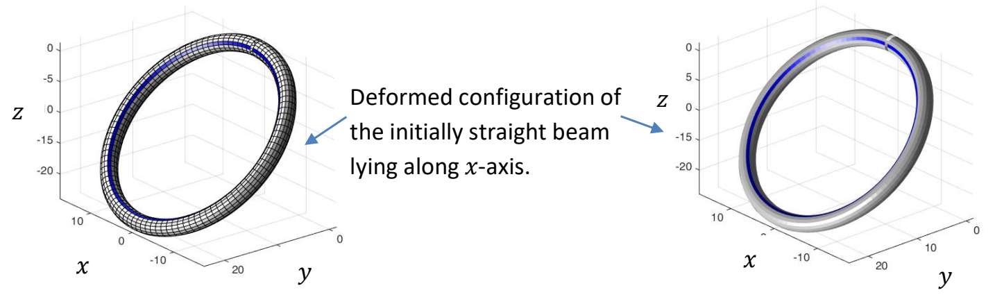
3 ( n − 1 ) unknowns . Example 1 L = 100 , G I t = 200 , E I y ˉ = E I z ˉ = E I = 400 L=100,\quad GI_t=200,\quad EI_{\bar y}=EI_{\bar z}=EI=400 L = 100 , G I t = 200 , E I y ˉ = E I z ˉ = E I = 400 C y = C z = 6.25 0.5 E I / L C_y=C_z=6.25\sqrt{0.5}EI/L C y = C z = 6.25 0.5 E I / L
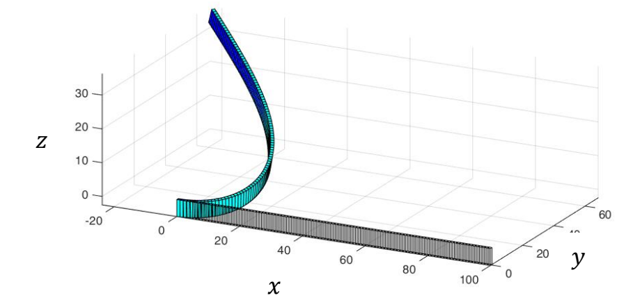
Figure 3. Deformed configuration of the initially straight beam lying along x x x Example 2 Clamped beam: L = 100 m m L=100\ \mathrm{mm} L = 100 mm E = 2 e 5 M P a E=2\mathrm{e}5\ \mathrm{MPa} E = 2 e 5 MPa
Load on the free end: X = − 33.33 N X=-33.33\ \mathrm{N} X = − 33.33 N Y = 16.67 N Y=16.67\ \mathrm{N} Y = 16.67 N Z = 23.33 N Z=23.33\ \mathrm{N} Z = 23.33 N C x = 0 C_x=0 C x = 0 C y = 0 C_y=0 C y = 0 C z = 0 C_z=0 C z = 0
Figure 4. Example 2: deformed cantilever beam.Maximum displacements (free end):
Matlab:
u = − 76.358 m m u=-76.358\ \mathrm{mm} u = − 76.358 mm v = 79.177 m m v=79.177\ \mathrm{mm} v = 79.177 mm w = 19.961 m m w=19.961\ \mathrm{mm} w = 19.961 mm
Ansys:
u = − 76.849 m m u=-76.849\ \mathrm{mm} u = − 76.849 mm v = 79.318 m m v=79.318\ \mathrm{mm} v = 79.318 mm w = 19.440 m m w=19.440\ \mathrm{mm} w = 19.440 mm
An Ansys macro can be downloaded here.
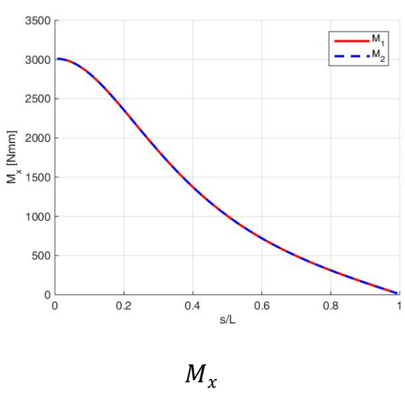
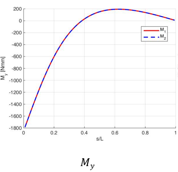
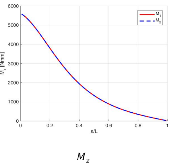
ZIP Example 2 — ANSYS macro Download ZIP The three moments in the global reference frame are checked in two ways:
M 1 = R T D κ ,
\boldsymbol{M}_1
=
\boldsymbol{R}^T\boldsymbol{D}\boldsymbol{\kappa},
M 1 = R T D κ , and
M 2 = { Z ( y n − y i ) − Y ( z n − z i ) + C x X ( z n − z i ) − Z ( x n − x i ) + C y Y ( x n − x i ) − X ( y n − y i ) + C z } .
\boldsymbol{M}_2
=
\left\{
\begin{array}{c}
Z(y_n-y_i)-Y(z_n-z_i)+C_x\\
X(z_n-z_i)-Z(x_n-x_i)+C_y\\
Y(x_n-x_i)-X(y_n-y_i)+C_z
\end{array}
\right\}.
M 2 = ⎩ ⎨ ⎧ Z ( y n − y i ) − Y ( z n − z i ) + C x X ( z n − z i ) − Z ( x n − x i ) + C y Y ( x n − x i ) − X ( y n − y i ) + C z ⎭ ⎬ ⎫ . Obviously, for correct results:
M 1 = M 2 .
\boldsymbol{M}_1=\boldsymbol{M}_2.
M 1 = M 2 . Figure 5. Example 2: global moment checks, M x M_x M x M y M_y M y M z M_z M z Example 3 L = 100 m m L=100\ \mathrm{mm} L = 100 mm G I t = 2000 2.6 , E I y ˉ = 1500 , E I z ˉ = 1000 , Z = 0.25 , C z = − 120 GI_t=\dfrac{2000}{2.6},\quad EI_{\bar y}=1500,\quad EI_{\bar z}=1000,\quad Z=0.25,\quad C_z=-120 G I t = 2.6 2000 , E I y ˉ = 1500 , E I z ˉ = 1000 , Z = 0.25 , C z = − 120
Figure 6. Example 3: deformed beam.
Figure 7. Example 3: interactive 3D view of the deformed beam.Deformed beam
Torsion moment and bending moments along the beam (local reference frame)
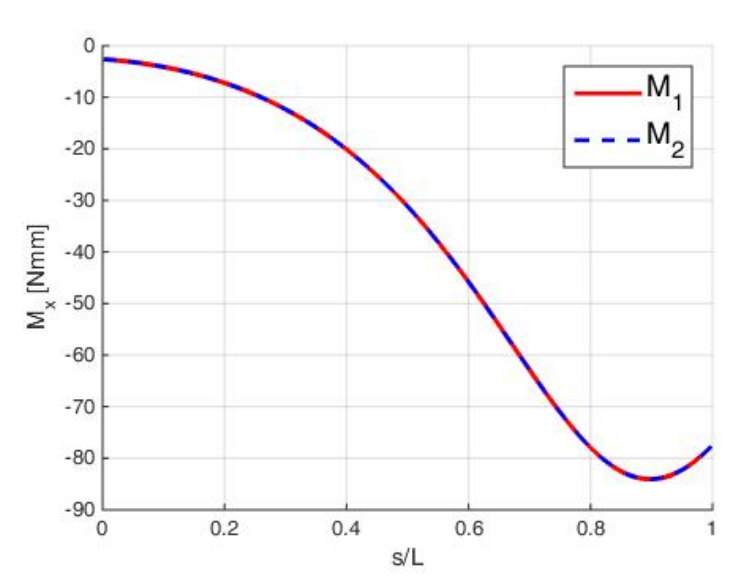
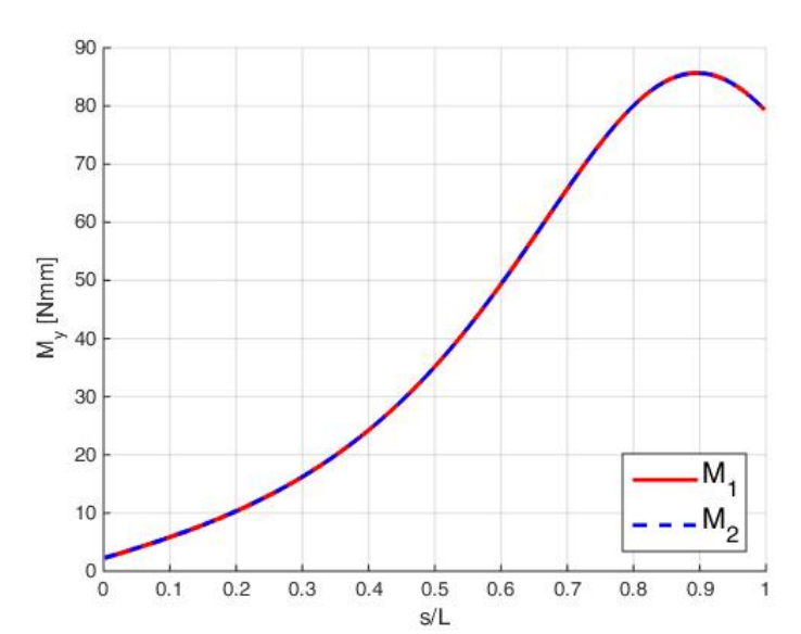
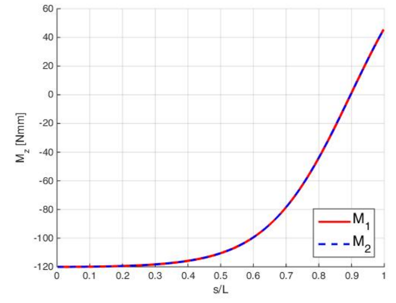
In the next diagrams, the three moments in the local reference frame are computed in two ways:
M ‾ 1 = D κ ,
\overline{\boldsymbol{M}}_1
=
\boldsymbol{D}\boldsymbol{\kappa},
M 1 = D κ , and
M ‾ 2 = R M .
\overline{\boldsymbol{M}}_2
=
\boldsymbol{R}\,\boldsymbol{M}.
M 2 = R M . Evidently, for correct results,
M ‾ 1 = M ‾ 2 .
\overline{\boldsymbol{M}}_1
=
\overline{\boldsymbol{M}}_2.
M 1 = M 2 . M x ˉ M_{\bar x} M x ˉ M y ˉ M_{\bar y} M y ˉ M z ˉ M_{\bar z} M z ˉ Figure 8. Example 3: local torsion and bending moment checks.References 1. Da Lozzo, E. C., Geometrically exact three-dimensional beam theory: modeling and FEM implementation for statics and dynamics analysis, Università degli Studi di Pavia, 2010.
2. Munteanu, M. Gh., Lobontiu, N., Nonlinear Finite Element Load-Displacement Model and Analysis of Circular-Axis Hinge, Self-Similar Mechanism With Large Out-of-Plane Motion, Journal of Mechanical Design, January 2022, Vol. 144(1)
PREVIOUS SECTION ← 22.1. Curvature tensor of a 3D slender beam. Euler–Bernoulli beam theory NEXT SECTION 23.1. 3D beam element. Euler–Bernoulli model →