Chapter 13

Euler–Almansi Strain Tensor

A current-configuration strain measure and its relation to the Green–Lagrange and linearized strain measures.

Current configurationFinite deformationInverse deformation gradientCauchy stress

01

Current-configuration kinematics

Another finite-strain measure is presented here in a form parallel to the Green–Lagrange strain tensor introduced in Chapter 10. Green–Lagrange strain measures changes in length with respect to the initial configuration, whereas Euler–Almansi strain measures them with respect to the current configuration.

The initial and current coordinates of a material point are:

x={xy},x^={x^y^}=x+u,u={uv}\boldsymbol{x}=\begin{Bmatrix}x\\[3pt]y\end{Bmatrix},\qquad \hat{\boldsymbol{x}}=\begin{Bmatrix}\hat{x}\\[3pt]\hat{y}\end{Bmatrix}=\boldsymbol{x}+\boldsymbol{u},\qquad \boldsymbol{u}=\begin{Bmatrix}u\\[3pt]v\end{Bmatrix}

The deformation gradient is:

F=x^x=[x^xx^yy^xy^y]=[1+uxuyvx1+vy]\boldsymbol{F}=\frac{\partial\hat{\boldsymbol{x}}}{\partial\boldsymbol{x}}=\begin{bmatrix}\dfrac{\partial\hat{x}}{\partial x}&\dfrac{\partial\hat{x}}{\partial y}\\[7pt]\dfrac{\partial\hat{y}}{\partial x}&\dfrac{\partial\hat{y}}{\partial y}\end{bmatrix}=\begin{bmatrix}1+\dfrac{\partial u}{\partial x}&\dfrac{\partial u}{\partial y}\\[7pt]\dfrac{\partial v}{\partial x}&1+\dfrac{\partial v}{\partial y}\end{bmatrix}
F=I2+ux,I2=[1001]\boldsymbol{F}=\boldsymbol{I}_2+\frac{\partial\boldsymbol{u}}{\partial\boldsymbol{x}},\qquad \boldsymbol{I}_2=\begin{bmatrix}1&0\\[3pt]0&1\end{bmatrix}

Therefore:

dx^=Fdxd\hat{\boldsymbol{x}}=\boldsymbol{F}\,d\boldsymbol{x}

To express the initial coordinates in terms of the current coordinates:

x=x^u\boldsymbol{x}=\hat{\boldsymbol{x}}-\boldsymbol{u}

Differentiation with respect to the current coordinates gives:

dx=F1dx^d\boldsymbol{x}=\boldsymbol{F}^{-1}d\hat{\boldsymbol{x}}
F1=xx^=[xx^xy^yx^yy^]=[1ux^uy^vx^1vy^]\boldsymbol{F}^{-1}=\frac{\partial\boldsymbol{x}}{\partial\hat{\boldsymbol{x}}}=\begin{bmatrix}\dfrac{\partial x}{\partial\hat{x}}&\dfrac{\partial x}{\partial\hat{y}}\\[7pt]\dfrac{\partial y}{\partial\hat{x}}&\dfrac{\partial y}{\partial\hat{y}}\end{bmatrix}=\begin{bmatrix}1-\dfrac{\partial u}{\partial\hat{x}}&-\dfrac{\partial u}{\partial\hat{y}}\\[7pt]-\dfrac{\partial v}{\partial\hat{x}}&1-\dfrac{\partial v}{\partial\hat{y}}\end{bmatrix}

The same inverse deformation gradient follows directly by inverting F\boldsymbol{F}:

F1=1Δ[1+vyuyvx1+ux]\boldsymbol{F}^{-1}=\frac{1}{\Delta}\begin{bmatrix}1+\dfrac{\partial v}{\partial y}&-\dfrac{\partial u}{\partial y}\\[7pt]-\dfrac{\partial v}{\partial x}&1+\dfrac{\partial u}{\partial x}\end{bmatrix}

where:

Δ=detF=1+ux+vy+uxvyvxuy\Delta=\det\boldsymbol{F}=1+\frac{\partial u}{\partial x}+\frac{\partial v}{\partial y}+\frac{\partial u}{\partial x}\frac{\partial v}{\partial y}-\frac{\partial v}{\partial x}\frac{\partial u}{\partial y}

Thus, the two equivalent forms are:

F1=[1ux^uy^vx^1vy^]=1Δ[1+vyuyvx1+ux]\boldsymbol{F}^{-1}=\begin{bmatrix}1-\dfrac{\partial u}{\partial\hat{x}}&-\dfrac{\partial u}{\partial\hat{y}}\\[7pt]-\dfrac{\partial v}{\partial\hat{x}}&1-\dfrac{\partial v}{\partial\hat{y}}\end{bmatrix}=\frac{1}{\Delta}\begin{bmatrix}1+\dfrac{\partial v}{\partial y}&-\dfrac{\partial u}{\partial y}\\[7pt]-\dfrac{\partial v}{\partial x}&1+\dfrac{\partial u}{\partial x}\end{bmatrix}

02

Euler–Almansi strain tensor

Using the current differential vector, the change in squared length is:

dx^Tdx^dxTdx=dx^Tdx^dx^TFTF1dx^d\hat{\boldsymbol{x}}^{T}d\hat{\boldsymbol{x}}-d\boldsymbol{x}^{T}d\boldsymbol{x}=d\hat{\boldsymbol{x}}^{T}d\hat{\boldsymbol{x}}-d\hat{\boldsymbol{x}}^{T}\boldsymbol{F}^{-T}\boldsymbol{F}^{-1}d\hat{\boldsymbol{x}}
dx^Tdx^dxTdx=dx^T(I2FTF1)dx^=2dx^Tedx^d\hat{\boldsymbol{x}}^{T}d\hat{\boldsymbol{x}}-d\boldsymbol{x}^{T}d\boldsymbol{x}=d\hat{\boldsymbol{x}}^{T}\left(\boldsymbol{I}_2-\boldsymbol{F}^{-T}\boldsymbol{F}^{-1}\right)d\hat{\boldsymbol{x}}=2d\hat{\boldsymbol{x}}^{T}\boldsymbol{e}\,d\hat{\boldsymbol{x}}

The Euler–Almansi strain tensor is therefore [1] [2]:

e=12(I2FTF1)\boxed{\boldsymbol{e}=\frac12\left(\boldsymbol{I}_2-\boldsymbol{F}^{-T}\boldsymbol{F}^{-1}\right)}

In terms of displacement gradients evaluated with respect to the current configuration:

e=12[ux^+(ux^)T(ux^)Tux^]\boldsymbol{e}=\frac12\left[\frac{\partial\boldsymbol{u}}{\partial\hat{\boldsymbol{x}}}+\left(\frac{\partial\boldsymbol{u}}{\partial\hat{\boldsymbol{x}}}\right)^{T}-\left(\frac{\partial\boldsymbol{u}}{\partial\hat{\boldsymbol{x}}}\right)^{T}\frac{\partial\boldsymbol{u}}{\partial\hat{\boldsymbol{x}}}\right]

Or, component by component:

{ex=ux^12(ux^)212(vx^)2ey=vy^12(uy^)212(vy^)2exy=12(uy^+vx^)12(ux^uy^+vx^vy^)\left\{\begin{aligned}e_x={}&\frac{\partial u}{\partial\hat{x}}-\frac12\left(\frac{\partial u}{\partial\hat{x}}\right)^2-\frac12\left(\frac{\partial v}{\partial\hat{x}}\right)^2\\[7pt]e_y={}&\frac{\partial v}{\partial\hat{y}}-\frac12\left(\frac{\partial u}{\partial\hat{y}}\right)^2-\frac12\left(\frac{\partial v}{\partial\hat{y}}\right)^2\\[7pt]e_{xy}={}&\frac12\left(\frac{\partial u}{\partial\hat{y}}+\frac{\partial v}{\partial\hat{x}}\right)-\frac12\left(\frac{\partial u}{\partial\hat{x}}\frac{\partial u}{\partial\hat{y}}+\frac{\partial v}{\partial\hat{x}}\frac{\partial v}{\partial\hat{y}}\right)\end{aligned}\right.

Euler–Almansi strains with engineering notation (γxy=2exy)(\gamma_{xy}=2e_{xy}) are:

{εx=ux^12(ux^)212(vx^)2εy=vy^12(uy^)212(vy^)2γxy=uy^+vx^ux^uy^vx^vy^\left\{\begin{aligned}\varepsilon_x={}&\frac{\partial u}{\partial\hat{x}}-\frac12\left(\frac{\partial u}{\partial\hat{x}}\right)^2-\frac12\left(\frac{\partial v}{\partial\hat{x}}\right)^2\\[7pt]\varepsilon_y={}&\frac{\partial v}{\partial\hat{y}}-\frac12\left(\frac{\partial u}{\partial\hat{y}}\right)^2-\frac12\left(\frac{\partial v}{\partial\hat{y}}\right)^2\\[7pt]\gamma_{xy}={}&\frac{\partial u}{\partial\hat{y}}+\frac{\partial v}{\partial\hat{x}}-\frac{\partial u}{\partial\hat{x}}\frac{\partial u}{\partial\hat{y}}-\frac{\partial v}{\partial\hat{x}}\frac{\partial v}{\partial\hat{y}}\end{aligned}\right.

The Euler–Almansi strain tensor predicts zero strain for any rigid-body motion [1]. This is the same essential rigid-motion invariance exhibited by Green–Lagrange strain.

03

Green–Lagrange and Euler–Almansi

The principal differences between the two strain measures are summarized in the comparison table:

Green–Lagrange strainsEuler–Almansi strains
Derivatives and integrals are evaluated with respect to the initial configuration, defined by x\boldsymbol{x}.Derivatives and integrals are evaluated with respect to the current configuration, defined by x^\hat{\boldsymbol{x}}.
dx^=Fdxd\hat{\boldsymbol{x}}=\boldsymbol{F}\,d\boldsymbol{x}
dx=F1dx^d\boldsymbol{x}=\boldsymbol{F}^{-1}d\hat{\boldsymbol{x}}
F=I2+ux\boldsymbol{F}=\boldsymbol{I}_2+\frac{\partial\boldsymbol{u}}{\partial\boldsymbol{x}}
F1=I2ux^\boldsymbol{F}^{-1}=\boldsymbol{I}_2-\frac{\partial\boldsymbol{u}}{\partial\hat{\boldsymbol{x}}}
EGL=12(FTFI2)\boldsymbol{E}_{GL}=\frac12\left(\boldsymbol{F}^{T}\boldsymbol{F}-\boldsymbol{I}_2\right)
eEA=12(I2FTF1)\boldsymbol{e}_{EA}=\frac12\left(\boldsymbol{I}_2-\boldsymbol{F}^{-T}\boldsymbol{F}^{-1}\right)
Engineering notation
{εx=u,x+12u,x2+12v,x2εy=v,y+12u,y2+12v,y2γxy=u,y+v,x+u,xu,y+v,xv,y\left\{\begin{aligned}\varepsilon_x={}&u_{,x}+\frac12u_{,x}^{2}+\frac12v_{,x}^{2}\\[4pt]\varepsilon_y={}&v_{,y}+\frac12u_{,y}^{2}+\frac12v_{,y}^{2}\\[4pt]\gamma_{xy}={}&u_{,y}+v_{,x}+u_{,x}u_{,y}+v_{,x}v_{,y}\end{aligned}\right.
{εx=u,x^12u,x^212v,x^2εy=v,y^12u,y^212v,y^2γxy=u,y^+v,x^u,x^u,y^v,x^v,y^\left\{\begin{aligned}\varepsilon_x={}&u_{,\hat{x}}-\frac12u_{,\hat{x}}^{2}-\frac12v_{,\hat{x}}^{2}\\[4pt]\varepsilon_y={}&v_{,\hat{y}}-\frac12u_{,\hat{y}}^{2}-\frac12v_{,\hat{y}}^{2}\\[4pt]\gamma_{xy}={}&u_{,\hat{y}}+v_{,\hat{x}}-u_{,\hat{x}}u_{,\hat{y}}-v_{,\hat{x}}v_{,\hat{y}}\end{aligned}\right.
One-dimensional case

The engineering axial strain and stretch ratio are:

ε=LL0L0=uL0,λ=LL0=1+ε\varepsilon=\frac{L-L_0}{L_0}=\frac{u}{L_0},\qquad \lambda=\frac{L}{L_0}=1+\varepsilon
EGL=L2L022L02=(L0+u)2L022L02E_{GL}=\frac{L^2-L_0^2}{2L_0^2}=\frac{(L_0+u)^2-L_0^2}{2L_0^2}
EGL=uL0+u22L02=12(λ21)E_{GL}=\frac{u}{L_0}+\frac{u^2}{2L_0^2}=\frac12\left(\lambda^2-1\right)
eEA=L2L022L2=L2(Lu)22L2e_{EA}=\frac{L^2-L_0^2}{2L^2}=\frac{L^2-(L-u)^2}{2L^2}
eEA=uLu22L2=12(1λ2)e_{EA}=\frac{u}{L}-\frac{u^2}{2L^2}=\frac12\left(1-\lambda^{-2}\right)

Here L0L_0 is the initial length, LL is the current length, and uu is the displacement of the free end. The exact relation is:

eEA=EGLλ2\boxed{e_{EA}=\frac{E_{GL}}{\lambda^2}}

This relation again reflects the use of the initial configuration for Green–Lagrange strain and of the current configuration for Euler–Almansi strain.

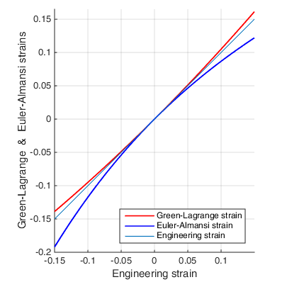
Comparison of Green–Lagrange, Euler–Almansi, and engineering axial strains
Figure 1. Green–Lagrange and Euler–Almansi strains compared with engineering axial strain.

MATLAB program used to draw the diagram above (copy and paste into MATLAB):

% Green_Almansi
em=0.15;
e=-em:0.001:em;
eG=e+e.^2/2;
e1=e./(1+e);
eA=e1-e1.^2/2;

figure(1), clf, hold on, grid on
axis('equal')
plot(e,eG,'r','linewidth',1.2)
plot(e,eA,'b','linewidth',1.2)
xlabel('Engineering strain')
ylabel('Green-Lagrange & Euler-Almansi strains')
plot(e,e)
legend('Green-Lagrange strain','Euler-Almansi strain',...
       'Engineering strain','Location','southeast')
axis([-0.15 0.15 -0.2 0.165])

04

Small-strain comparison

For very small strains:

EGLeEAεE_{GL}\approx e_{EA}\approx\varepsilon

For steel, for example, elastic strain is usually smaller than approximately 0.010.01, provided that no plasticity occurs.

Over the interval:

ε[0.05,0.05]\varepsilon\in[-0.05,0.05]

the difference from engineering strain is approximately 23%2\text{–}3\% for Green–Lagrange strain and approximately 78%7\text{–}8\% for Euler–Almansi strain.

Current-configuration stress interpretation

When the Euler–Almansi strains are small, the usual linear elastic Hooke law can be applied in the current configuration, providing a very good approximation of the Cauchy stresses.

05

Strain and stress measures

The table below summarizes stress and strain measures commonly associated with the formulations considered in this website. More general finite-strain formulations may use other stress and strain measures [3] [4].

Type of analysisDescriptionFormulationStress and strain measures
Material nonlinearity onlyInfinitesimal displacements and strains; the stress–strain relation is nonlinearLinearized strain and Cauchy stress
Large displacements and rotations, but small strainsThe stress–strain relation may be linear or nonlinearTotal Lagrangian (TL)Second Piola–Kirchhoff stress and Green–Lagrange strain
Updated Lagrangian (UL)Cauchy stress and Euler–Almansi strain
Large displacements, rotations, and strainsThe stress–strain relation may be linear or nonlinearTotal Lagrangian (TL)Second Piola–Kirchhoff stress and Green–Lagrange strain
Updated Lagrangian (UL)Cauchy stress and logarithmic strain

06

References

  1. Green Strain, ContinuumMechanics.org.

  2. Nam-Ho Kim, Introduction to Nonlinear Finite Element Analysis, Springer, 2015.

  3. Eleni Chatzi, The Finite Element Method for the Analysis of Non-Linear and Dynamic Systems, ETH Zürich, Lecture 3, 15 October 2015.

  4. Finite strain theory, Wikipedia.