14. Cauchy, First Piola–Kirchhoff, and Second Piola–Kirchhoff Stress Tensors

Three-dimensional kinematics

Although many structures can be modeled as two-dimensional, real bodies are three-dimensional. To introduce the Piola–Kirchhoff stress measures and the transformation of oriented areas between the reference and current configurations, we therefore consider the general three-dimensional case.

The reference coordinates, displacement vector, and current coordinates of a material point are:

\boldsymbol{x}=\begin{Bmatrix}x\\[3pt]y\\[3pt]z\end{Bmatrix},\qquad \boldsymbol{u}=\begin{Bmatrix}u\\[3pt]v\\[3pt]w\end{Bmatrix},\qquad \hat{\boldsymbol{x}}=\boldsymbol{x}+\boldsymbol{u}

The displacement gradient is denoted by:

\nabla\boldsymbol{u}=\frac{\partial\boldsymbol{u}}{\partial\boldsymbol{x}}=\begin{bmatrix}\dfrac{\partial u}{\partial x}&\dfrac{\partial u}{\partial y}&\dfrac{\partial u}{\partial z}\\[6pt]\dfrac{\partial v}{\partial x}&\dfrac{\partial v}{\partial y}&\dfrac{\partial v}{\partial z}\\[6pt]\dfrac{\partial w}{\partial x}&\dfrac{\partial w}{\partial y}&\dfrac{\partial w}{\partial z}\end{bmatrix}

The deformation gradient is:

\boldsymbol{F}=\frac{\partial\hat{\boldsymbol{x}}}{\partial\boldsymbol{x}}=\begin{bmatrix}\dfrac{\partial\hat{x}}{\partial x}&\dfrac{\partial\hat{x}}{\partial y}&\dfrac{\partial\hat{x}}{\partial z}\\[6pt]\dfrac{\partial\hat{y}}{\partial x}&\dfrac{\partial\hat{y}}{\partial y}&\dfrac{\partial\hat{y}}{\partial z}\\[6pt]\dfrac{\partial\hat{z}}{\partial x}&\dfrac{\partial\hat{z}}{\partial y}&\dfrac{\partial\hat{z}}{\partial z}\end{bmatrix}=\boldsymbol{I}_3+\nabla\boldsymbol{u}

An infinitesimal material vector transforms according to:

d\hat{\boldsymbol{x}}=\boldsymbol{F}\,d\boldsymbol{x}

The Green–Lagrange strain tensor is:

\boldsymbol{E}=\frac12\left(\boldsymbol{F}^{T}\boldsymbol{F}-\boldsymbol{I}_3\right)

Or, using the displacement gradient:

\boldsymbol{E}=\frac12\left[\nabla\boldsymbol{u}+\left(\nabla\boldsymbol{u}\right)^T+\left(\nabla\boldsymbol{u}\right)^T\nabla\boldsymbol{u}\right]

Using engineering notation, its six independent components are:

\left\{\begin{aligned}E_x={}&u_{,x}+\frac12\left(u_{,x}^{2}+v_{,x}^{2}+w_{,x}^{2}\right)\\[4pt]E_y={}&v_{,y}+\frac12\left(u_{,y}^{2}+v_{,y}^{2}+w_{,y}^{2}\right)\\[4pt]E_z={}&w_{,z}+\frac12\left(u_{,z}^{2}+v_{,z}^{2}+w_{,z}^{2}\right)\\[4pt]\gamma_{xy}={}&u_{,y}+v_{,x}+u_{,x}u_{,y}+v_{,x}v_{,y}+w_{,x}w_{,y}\\[4pt]\gamma_{yz}={}&v_{,z}+w_{,y}+u_{,y}u_{,z}+v_{,y}v_{,z}+w_{,y}w_{,z}\\[4pt]\gamma_{zx}={}&w_{,x}+u_{,z}+u_{,z}u_{,x}+v_{,z}v_{,x}+w_{,z}w_{,x}\end{aligned}\right.

Volume deformation

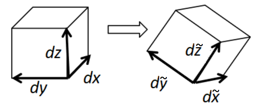
Consider an elementary rectangular parallelepiped with reference edge lengths $dx$ , $dy$ , and $dz$ . After deformation, its faces are generally parallelograms [1] [2].

Reference rectangular parallelepiped and its deformed configuration — **Figure 1.** Differential volume in the reference and current configurations.

The reference volume is:

dV_0=dx\,dy\,dz

If $\boldsymbol{f}_1$ , $\boldsymbol{f}_2$ , and $\boldsymbol{f}_3$ are the columns of $\boldsymbol{F}$ , the three current edge vectors are:

d\hat{\boldsymbol{x}}=\boldsymbol{F}\begin{Bmatrix}dx\\0\\0\end{Bmatrix}=\boldsymbol{f}_1\,dx,\qquad d\hat{\boldsymbol{y}}=\boldsymbol{F}\begin{Bmatrix}0\\dy\\0\end{Bmatrix}=\boldsymbol{f}_2\,dy,\qquad d\hat{\boldsymbol{z}}=\boldsymbol{F}\begin{Bmatrix}0\\0\\dz\end{Bmatrix}=\boldsymbol{f}_3\,dz

The current volume follows from the scalar triple product:

dV=d\hat{\boldsymbol{x}}\mathbin{\boldsymbol{\cdot}}\left(d\hat{\boldsymbol{y}}\mathbin{\boldsymbol{\times}}d\hat{\boldsymbol{z}}\right)=\det\begin{bmatrix}d\hat{x}_x&d\hat{y}_x&d\hat{z}_x\\d\hat{x}_y&d\hat{y}_y&d\hat{z}_y\\d\hat{x}_z&d\hat{y}_z&d\hat{z}_z\end{bmatrix}

dV=\det\boldsymbol{F}\,dx\,dy\,dz=\Delta\,dV_0

In many finite-strain texts, the determinant of the deformation gradient is denoted $J=\det\boldsymbol{F}$ . To avoid confusion here with the isoparametric Jacobian $\boldsymbol{J}$ , we shall use $\Delta$ :

\boxed{\Delta=\det\boldsymbol{F}}

The volumetric strain is therefore:

\varepsilon_V=\frac{dV-dV_0}{dV_0}=\Delta-1

Cauchy stress and first Piola–Kirchhoff stress

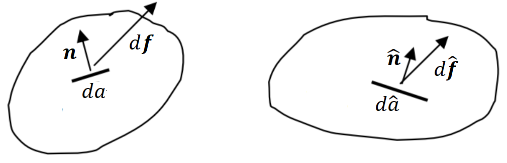
The reference configuration describes the body before deformation; the current external and internal forces act on the deformed body. The area element $d\boldsymbol{a}$ in the reference configuration is therefore used only as a reference measure.

The corresponding material surface element in the current configuration is $d\hat{\boldsymbol{a}}$ . The two oriented area elements describe the same material surface before and after deformation. During deformation, both its area and its orientation may change.

The physical infinitesimal force $d\boldsymbol{f}$ transmitted through this surface belongs to the current configuration. The Cauchy stress tensor $\boldsymbol{\sigma}$ relates this force to the current oriented area:

d\boldsymbol{f}=\boldsymbol{\sigma}\,d\hat{\boldsymbol{a}}

The first Piola–Kirchhoff stress tensor $\boldsymbol{P}$ (PK1) is introduced by referring the same current force to the corresponding area in the reference configuration:

d\boldsymbol{f}=\boldsymbol{P}\,d\boldsymbol{a}

Therefore:

\boldsymbol{\sigma}\,d\hat{\boldsymbol{a}}=\boldsymbol{P}\,d\boldsymbol{a}

Thus, no force is being applied to the undeformed configuration: the reference area is used only to measure the same force acting in the current configuration. The two expressions represent the same physical current force using two different oriented-area measures.

Force and oriented area vectors in the reference and current configurations — **Figure 2.** The same differential force is related to a reference area by PK1 and to a current area by Cauchy stress.

Nanson’s formula

Consider an infinitesimal oriented area $d\boldsymbol{a}$ . By translating it through an arbitrary infinitesimal vector $d\boldsymbol{r}$ , a differential volume is generated:

dV_0=d\boldsymbol{r}\mathbin{\boldsymbol{\cdot}}d\boldsymbol{a}

In the current configuration:

dV=d\hat{\boldsymbol{r}}\mathbin{\boldsymbol{\cdot}}d\hat{\boldsymbol{a}},\qquad d\hat{\boldsymbol{r}}=\boldsymbol{F}\,d\boldsymbol{r}

Because $dV=\Delta\,dV_0$ :

\left(\boldsymbol{F}\,d\boldsymbol{r}\right)\mathbin{\boldsymbol{\cdot}}d\hat{\boldsymbol{a}}=\Delta\,d\boldsymbol{r}\mathbin{\boldsymbol{\cdot}}d\boldsymbol{a}

For an arbitrary $d\boldsymbol{r}$ , this gives:

\boldsymbol{F}^{T}d\hat{\boldsymbol{a}}=\Delta\,d\boldsymbol{a}

Therefore, Nanson’s formula is:

\boxed{d\hat{\boldsymbol{a}}=\Delta\,\boldsymbol{F}^{-T}d\boldsymbol{a}}

Equating the force described by Cauchy stress and PK1, then using Nanson’s formula:

\boldsymbol{P}\,d\boldsymbol{a}=\boldsymbol{\sigma}\,d\hat{\boldsymbol{a}}=\Delta\,\boldsymbol{\sigma}\boldsymbol{F}^{-T}d\boldsymbol{a}

The direct and inverse transformations are:

\boxed{\boldsymbol{P}=\Delta\,\boldsymbol{\sigma}\boldsymbol{F}^{-T}},\qquad \boxed{\boldsymbol{\sigma}=\frac{1}{\Delta}\boldsymbol{P}\boldsymbol{F}^{T}}

Second Piola–Kirchhoff stress

The Cauchy stress is symmetric, but the deformation gradient is generally not. Consequently, PK1 is generally non-symmetric. The second Piola–Kirchhoff stress does not have the direct physical interpretation of the Cauchy stress, but there are important reasons for using it as a stress measure.

The second Piola–Kirchhoff stress tensor $\boldsymbol{S}$ (PK2) is defined by pulling PK1 back to the reference configuration:

\boxed{\boldsymbol{S}=\boldsymbol{F}^{-1}\boldsymbol{P}}

Using the PK1–Cauchy relation:

\boxed{\boldsymbol{S}=\Delta\,\boldsymbol{F}^{-1}\boldsymbol{\sigma}\boldsymbol{F}^{-T}}

The corresponding Cauchy transformation is:

\boxed{\boldsymbol{\sigma}=\frac{1}{\Delta}\boldsymbol{F}\boldsymbol{S}\boldsymbol{F}^{T}}

Since the Cauchy stress tensor is symmetric, the second Piola–Kirchhoff stress tensor is also symmetric:

\boldsymbol{S}^{T}=\left(\Delta\,\boldsymbol{F}^{-1}\boldsymbol{\sigma}\boldsymbol{F}^{-T}\right)^T=\Delta\,\boldsymbol{F}^{-1}\boldsymbol{\sigma}^{T}\boldsymbol{F}^{-T}=\boldsymbol{S}

This is one of the reasons why PK2 is particularly convenient in Total Lagrangian formulations.

Cauchy stressCurrent force / current area

First Piola–Kirchhoff stressCurrent force / reference area

Second Piola–Kirchhoff stressBoth force and area are pulled back to the reference configuration

This simple interpretation also explains why PK1 is generally non-symmetric, while PK2 is symmetric and particularly convenient in Total Lagrangian formulations.

Saint Venant–Kirchhoff material

A linear relation is assumed between Green–Lagrange strain and second Piola–Kirchhoff stress because both measures refer to the reference configuration [1] [3]:

\boldsymbol{S}=\boldsymbol{D}\,\boldsymbol{E}

In three-dimensional engineering notation:

\begin{Bmatrix}S_x\\S_y\\S_z\\T_{xy}\\T_{yz}\\T_{zx}\end{Bmatrix}=\boldsymbol{D}_{3D}\begin{Bmatrix}E_x\\E_y\\E_z\\\gamma_{xy}\\\gamma_{yz}\\\gamma_{zx}\end{Bmatrix}

\boldsymbol{D}_{3D}=\frac{E}{(1+\nu)(1-2\nu)}\begin{bmatrix}1-\nu&\nu&\nu&0&0&0\\\nu&1-\nu&\nu&0&0&0\\\nu&\nu&1-\nu&0&0&0\\0&0&0&\dfrac{1-2\nu}{2}&0&0\\0&0&0&0&\dfrac{1-2\nu}{2}&0\\0&0&0&0&0&\dfrac{1-2\nu}{2}\end{bmatrix}

For a two-dimensional plane-stress state:

\begin{Bmatrix}S_x\\S_y\\T_{xy}\end{Bmatrix}=\boldsymbol{D}_{\mathrm{ps}}\begin{Bmatrix}E_x\\E_y\\\gamma_{xy}\end{Bmatrix},\qquad \boldsymbol{D}_{\mathrm{ps}}=\frac{E}{1-\nu^2}\begin{bmatrix}1&\nu&0\\\nu&1&0\\0&0&\dfrac{1-\nu}{2}\end{bmatrix}

For infinitesimal strains and rotations, this relation reduces to the usual linear elastic Hooke law. It is particularly useful for problems involving large displacements and rotations but small strains.

Range of applicability

The Saint Venant–Kirchhoff model is generally not suitable for large elastic strains.

Example 1: uniaxial tension

A cantilever beam has length $L=400\ \mathrm{mm}$ , rectangular cross-section $5\ \mathrm{mm}\times60\ \mathrm{mm}$ , Young’s modulus $E=1000\ \mathrm{MPa}$ , and Poisson’s ratio $\nu=0.3$ . A tensile force $F=24000\ \mathrm{N}$ is applied at the free end. The mesh contains 24 elements along the length and 4 elements through the height; mesh refinement has no influence in this homogeneous pure-tension case.

Reference coordinate axes — **Figure 3.** Geometry, mesh, boundary conditions, and tensile loading for Example 1.

Finite element mesh and distributed tensile loading for Example 1 — **Figure 3.** Geometry, mesh, boundary conditions, and tensile loading for Example 1.

The small-deformation linear result is:

\sigma_x=\frac{F}{A}=\frac{24000}{5\cdot60}=80\ \mathrm{MPa},\qquad \varepsilon_x=\frac{\sigma_x}{E}=0.08

The Total Lagrangian solution of Section 12.2, using Green–Lagrange strain and PK2 stress, gives:

S_x=74.625\ \mathrm{MPa},\qquad E_x=0.074625

Why the strain is relatively large

The strain in this example is intentionally larger than in the previous chapters, in order to make the differences between the Cauchy, first Piola–Kirchhoff and second Piola–Kirchhoff stresses clearly visible. Therefore, the example should be regarded mainly as a simple illustration of the relations between the different stress measures.

For the homogeneous uniaxial state, the PK2 tensor is:

\boldsymbol{S}=\begin{bmatrix}74.625&0&0\\0&0&0\\0&0&0\end{bmatrix}\ \mathrm{MPa}

The axial elongation and transverse contractions give:

u_{,x}=\frac{\Delta L}{L}=\frac{28.812}{400}=0.0720,\qquad v_{,y}=w_{,z}=-0.02264

Here, $\Delta L=28.812\ \mathrm{mm}$ is the elongation obtained from the nonlinear Total Lagrangian analysis of Section 12.2, in which the deformation is described by the Green–Lagrange strain measure. The initial beam length is $L=400\ \mathrm{mm}$ .

Thus, the deformation gradient is:

\boldsymbol{F}=\begin{bmatrix}1.0720&0&0\\0&0.97736&0\\0&0&0.97761\end{bmatrix}

The Green–Lagrange tensile strain is recovered directly:

E_x=\frac{\Delta L}{L}+\frac{(\Delta L)^2}{2L^2}=0.074625

Substitution of this elongation into the Green–Lagrange strain relation gives exactly the strain obtained in the finite-element solution.

Since $\boldsymbol{P}=\boldsymbol{F}\boldsymbol{S}$ , the axial PK1 stress is:

P_x=\left(1+u_{,x}\right)S_x=1.0720\cdot74.625=80\ \mathrm{MPa}

For this homogeneous uniaxial case, the PK1 value follows exactly from the PK2–PK1 transformation.

The volume ratio is:

\Delta=\det\boldsymbol{F}=1.0243

The Cauchy stress obtained from PK2 is:

\sigma_x=\frac{1}{\Delta}(1.0720)S_x(1.0720)=83.72\ \mathrm{MPa}

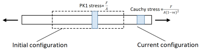
PK1 stress on the reference area and Cauchy stress on the contracted current area — **Figure 4.** PK1 uses the reference area, whereas Cauchy stress uses the contracted current area.

An independent calculation from force divided by the current cross-sectional area gives:

\sigma_x=\frac{F}{A_{\mathrm{current}}}=\frac{24000}{5\cdot60\left(1-0.3\cdot0.074625\right)^2}=83.72\ \mathrm{MPa}

This provides an independent check of the PK2-to-Cauchy transformation. For smaller strains, the numerical differences between these stress measures would rapidly decrease, as expected.

For a few additional remarks by Chiara on the physical interpretation of the second Piola–Kirchhoff stress and its relation to equilibrium, click here.

Plane stress and thickness change

Although a plane-stress problem is modeled in 2D, the body is still three-dimensional. Therefore, when stress measures are transformed, the change in thickness must also be taken into account.

The in-plane deformation gradient is:

\boldsymbol{F}_{2D}=\begin{bmatrix}1+u_{,x}&u_{,y}\\v_{,x}&1+v_{,y}\end{bmatrix}

For a plane-stress state and small strains, the thickness strain due to Poisson contraction can be approximated by:

\varepsilon_z=-\frac{\nu}{1-\nu}\left(\varepsilon_x+\varepsilon_y\right)\approx-\frac{\nu}{1-\nu}\left(u_{,x}+v_{,y}\right)

where the second form follows from the small-strain approximations $\varepsilon_x\approx u_{,x}$ and $\varepsilon_y\approx v_{,y}$ .

Consequently, the current thickness is approximated by:

h_{\mathrm{cur}}\approx(1+\varepsilon_z)h\approx\left[1-\frac{\nu}{1-\nu}\left(u_{,x}+v_{,y}\right)\right]h

The corresponding three-dimensional determinant required in the stress transformations is:

\Delta\approx\det\begin{bmatrix}1+u_{,x}&u_{,y}&0\\v_{,x}&1+v_{,y}&0\\0&0&1-\dfrac{\nu}{1-\nu}\left(\varepsilon_x+\varepsilon_y\right)\end{bmatrix}

or, using the small-strain approximation directly in terms of the displacement gradients:

\Delta\approx\det\begin{bmatrix}1+u_{,x}&u_{,y}&0\\v_{,x}&1+v_{,y}&0\\0&0&1-\dfrac{\nu}{1-\nu}\left(u_{,x}+v_{,y}\right)\end{bmatrix}

This thickness relation is a small-strain approximation; it is not a general exact relation for finite elastic strains.

References

Nam-Ho Kim, Introduction to Nonlinear Finite Element Analysis, Springer, 2015.
P. A. Kelly, Solid Mechanics Part III, Section 3.5 — Stress Measures for Large Deformations, University of Auckland.
Eleni Chatzi, Konstantinos Tatsis, and Konstantinos Agathos, Introduction to Geometrical Non-linearities, ETH Zürich, Lecture 2, 2021.