Polar decomposition, Hencky strain, Biot strain

01

Strain measures in ANSYS

ANSYS uses an updated Lagrangian formulation for geometric nonlinearities activated with NLGEOM,ON. For large-strain analyses, it uses logarithmic strain, also called Hencky strain or true strain. When rotations are large but the mechanical strains remain small, Biot strain, or small engineering strain, is used together with a corotational formulation [1].

The purpose of this section is to introduce the minimum kinematic background needed for the Hencky- and Biot-based formulations that follow. The physical meaning of each tensor is emphasized, because the expressions involve operations—such as the square root and logarithm of a matrix—that may be unfamiliar at first.

02

Deformation and rigid-body motion

As in Chapter 10, the position vector in the initial, undeformed configuration is $\boldsymbol{x}$, the position vector in the current, deformed configuration is $\widehat{\boldsymbol{x}}$, and the displacement vector is $\boldsymbol{u}$:

All displacement derivatives are evaluated with respect to the coordinates of the undeformed configuration. The displacement-gradient notation introduced in Chapter 10 is:

In two dimensions, its component form is:

The deformation gradient is therefore:

Written in components:

The deformation gradient maps an infinitesimal material vector from the undeformed configuration to the deformed configuration:

The right Cauchy–Green tensor is defined by [2]:

It contains the change in length and angle produced by the deformation, but it does not contain a superimposed rigid-body rotation. In the absence of strain:

The Green–Lagrange strain tensor is:

Consequently, a strain-free motion also gives:

A rigid translation is constant over the body. It disappears when derivatives are taken and therefore does not enter $\boldsymbol{F}$. For a finite rigid-body rotation through the angle $\theta$:

The deformation gradient of this rigid rotation is $\boldsymbol{F}=\boldsymbol{R}$. Since $\boldsymbol{R}^{T}\boldsymbol{R}=\boldsymbol{I}_2$:

More generally, if a rotation is superimposed on a deformation, the new deformation gradient is $\boldsymbol{R}\boldsymbol{F}$, while the right Cauchy–Green tensor remains unchanged:

The tensor $\boldsymbol{C}$ is also positive definite when $\boldsymbol{F}$ is nonsingular. Indeed, for any non-zero vector $\boldsymbol{a}$:

This property is important because it guarantees positive principal stretches and permits the unique matrix square root introduced next.

03

Right stretch and polar decomposition

The right stretch tensor $\boldsymbol{U}$ is defined by:

Equivalently:

This is a matrix square root, not the separate square root of every matrix entry. The tensor $\boldsymbol{U}$ is the matrix whose product with itself gives $\boldsymbol{C}$. Because $\boldsymbol{C}$ is symmetric positive definite, the physically relevant symmetric positive-definite square root exists and is unique.

In MATLAB, the matrix square root is computed by:

The function sqrtm computes the matrix square root. It must not be confused with applying the scalar square root separately to each entry.

If $\boldsymbol{F}$ is nonsingular, it can be decomposed uniquely into an orthogonal rotation tensor $\boldsymbol{R}$ and the symmetric positive-definite right stretch tensor $\boldsymbol{U}$ [2] [3]:

This factorization is called the polar decomposition. The tensor $\boldsymbol{U}$ first produces the stretch or deformation, and $\boldsymbol{R}$ subsequently rotates the stretched configuration. Since $\boldsymbol{R}^{T}\boldsymbol{R}=\boldsymbol{I}_2$:

To see the geometrical meaning, consider an infinitesimal square around a point $A$ in a two-dimensional body. Its sides are initially parallel to the global axes. Because the square is infinitesimal, the deformation of its points is described locally by $d\widehat{\boldsymbol{x}}=\boldsymbol{F}\,d\boldsymbol{x}$. We may translate the square so that point $A$ coincides with the origin; this rigid translation does not deform the square.

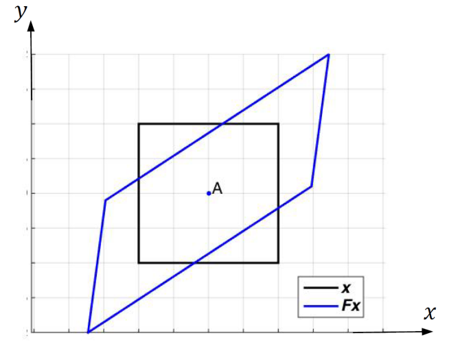
In Figure 1, the black square becomes the blue parallelogram. Its side lengths change, its right angles generally change, and the configuration also rotates.

Now consider an infinitesimal square whose sides are aligned with the principal directions of $\boldsymbol{U}$. In this special orientation the square changes its side lengths, but its right angles remain right angles. The result is a rectangle that is then rotated:

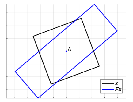
The complete motion can therefore be understood in two stages:

04

Principal stretches and left stretch

The symmetric tensor $\boldsymbol{U}$ has mutually orthogonal eigenvectors. In two dimensions, let:

where $\boldsymbol{q}_1$ and $\boldsymbol{q}_2$ are unit eigenvectors of $\boldsymbol{U}$. These eigenvectors define the two principal directions of stretch. The eigenvalue decomposition is:

Equivalently, in the principal frame:

The eigenvalues $\lambda_1$ and $\lambda_2$ are principal stretch ratios. A stretch ratio is not a strain. It is the ratio between the final and initial lengths measured in a principal direction:

Thus, $\lambda_i=1$ means no change in length, $\lambda_i>1$ means extension, and $\lambda_i<1$ means contraction.

The matrix $\boldsymbol{U}$ deforms the sides of the infinitesimal square while preserving the right angles when the sides are aligned with the principal directions. The changes in length are described by $\lambda_1$ and $\lambda_2$. This explains the name right stretch tensor.

The word right refers to the fact that $\boldsymbol{U}$ appears on the right-hand side of $\boldsymbol{R}$ in the polar decomposition

Similarly, $\boldsymbol{V}$ is called the left stretch tensor because it appears on the left-hand side of $\boldsymbol{R}$ in the equivalent polar decomposition

The matrix $\boldsymbol{R}$ then rotates the rectangle obtained after the action of $\boldsymbol{U}$.

Figure 3 shows the black initial square, the red dashed rectangle obtained after the action of $\boldsymbol{U}$, and the blue final configuration obtained after the rotation $\boldsymbol{R}$. The principal directions determine the sides along which the stretches $\lambda_1$ and $\lambda_2$ act. In three dimensions, the entries of $\boldsymbol{Q}$ may be interpreted as the direction cosines of the principal directions relative to the global axes.

There is also a left stretch tensor $\boldsymbol{V}$. The right and left stretch tensors are defined in parallel by:

The two tensors are related through the rotation:

Both $\boldsymbol{U}$ and $\boldsymbol{V}$ are symmetric positive-definite tensors. The following sections use the material description based on $\boldsymbol{U}$.

05

Numerical example

Consider the following deformation gradient:

The right Cauchy–Green tensor is:

The right stretch tensor, rotation tensor, principal stretches, and left stretch tensor are:

One possible orthonormal eigenvector matrix is:

The sign of an eigenvector may be reversed without changing its direction or the decomposition. The following MATLAB program, polar_decomposition_2d.m, illustrates the polar decomposition and the deformation of the infinitesimal square:

%*** polar_decomposition_2d ***
clc
clear

F=[1.062   0.0125
   0.110   0.947]

% Green-Lagrange strain tensor
E=1/2*(F'*F-eye(2))

% Infinitesimal square
xy=[-1 1 1 -1 -1; -1 -1 1 1 -1];

% Polar decomposition: F=R*U
C=F'*F
U=sqrtm(C)
R=F*inv(U)
[Q,Lambda]=eig(U)
V=R*U*R'

% Hencky and Biot strain tensors
eH=logm(U)
eB=U-eye(2)

% Square aligned with the principal directions
xyq=Q*xy;
xys=U*xyq;
xyr=R*xys;

figure(1)
clf, hold on, axis('equal'), grid on
title(strcat('\lambda_1=',num2str(Lambda(1,1)),...
 ', \lambda_2=',num2str(Lambda(2,2))))
plot(xyq(1,:),xyq(2,:),'k','linewidth',2)
plot(xys(1,:),xys(2,:),'--r','linewidth',1)
plot(xyr(1,:),xyr(2,:),'b','linewidth',2)
plot(0,0,'b.','MarkerSize',15)
lh=legend('x','Ux','Fx=RUx','Point A','location','southeast');
set(lh,'FontSize',15)
tx=text(0.05,0.06,'A');
set(tx,'FontSize',15)

06

Three-dimensional extension

In three dimensions, the deformation gradient and the stretch tensors are $3\times3$ matrices. In the principal frame, the right stretch tensor has the simple diagonal form:

The local volume change is governed by the determinant of the deformation gradient. Therefore, the volumetric strain is (see Chapter 14):

The relevant determinant relations are:

For the right Cauchy–Green tensor:

07

Hencky and Biot strains

Hencky strain is another strain measure. It is also called logarithmic strain or true strain and is defined by:

Here the shear components are written using engineering notation, so the tensorial shear strains are $\gamma_{ij}/2$.

Both Hencky and Biot strains are symmetric second-order strain tensors.

Because $\boldsymbol{U}$ is symmetric positive definite, it has positive eigenvalues and therefore a unique real symmetric principal matrix logarithm [4] [5]. In MATLAB, the matrix logarithm is computed by:

The function logm computes the matrix logarithm. As with the matrix square root, this is not obtained by taking the scalar logarithm of every entry separately.

A practical definition follows directly from the eigenvalue decomposition:

The matrix logarithm is then:

In two dimensions:

Thus, in the principal frame, the ordinary scalar logarithm is applied to each positive principal stretch ratio. The result is then transformed back to the original frame. This makes the logarithm of a matrix a concrete and well-defined operation rather than a symbolic analogy.

When $\boldsymbol{U}$ is sufficiently close to $\boldsymbol{I}$, its logarithm can also be represented by the Maclaurin series [4] [5]:

Biot strain is an independent strain measure defined by:

For small strains, $\boldsymbol{U}$ is close to $\boldsymbol{I}$, and the higher-order terms of the logarithm become small. Consequently:

The principal Hencky and Biot strains have particularly simple forms:

Further engineering-oriented discussion of these strain measures can be found in [6].

08

One-dimensional comparison

Finally, consider a prismatic bar with initial length $L_0$. If the end displacement is $u$, the final length is $L=L_0+u$, and the stretch ratio is:

The engineering strain is:

The Green–Lagrange strain is:

The Euler–Almansi strain is:

The Hencky strain is:

The Biot strain is:

In one dimension, the Biot strain coincides exactly with the engineering strain, while all these strain measures approach each other for small strains [7].

09

References

1. Ansys Inc., ANSYS Mechanical APDL Theory Reference, Release 2026 R1, 2026.

2. Nam-Ho Kim, Introduction to Nonlinear Finite Element Analysis, Springer, 2015.

3. Continuum Mechanics, ContinuumMechanics.org.

4. Nick Higham, What Is the Matrix Logarithm?

5. Logarithm of a Matrix, Wikipedia.

6. Antonio Bilotta, Structural Engineering.

7. Strain (Mechanics), Wikipedia.