21.2. Tait-Bryan angles

Tait-Bryan angles

Tait-Bryan angles are a particular three-angle parametrization of rotations, closely related to Euler angles [1]. They are utilised in aerospace applications to depict the aircraft's orientation in relation to the 3D world frame. In this site, the Tait-Bryan angles are utilised to define the position of a 3D beam, or only of an infinitely small segment $ds$ of a beam, in the global 3D reference frame.

The local reference frame of a beam, or of an infinitely short segment of a curved beam, is defined like this: $\bar x$ -axis is the locus of the centres of gravity of its cross-sections, $\bar y$ -axis and $\bar z$ -axis are the principal axes of its cross-section. The Tait-Bryan angles are presented in the figures below, [1].

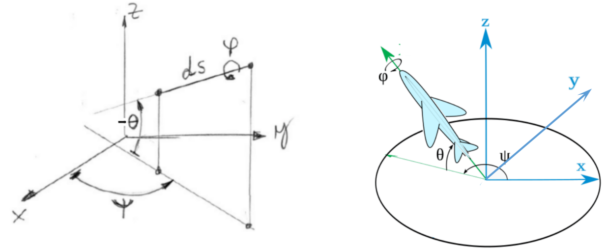
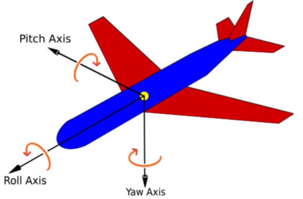
**Figure 1.** Tait-Bryan angles for a beam segment and an aircraft.

We assume that the local reference frame is obtained as follows: initially the local frame coincides with the global one: the beam lies on the global $x$ -axis and global $y$ -axis and $z$ -axis are parallel to the principal axes of its cross-sections. We apply three consecutive rotations. On this site, we prefer the order yaw, pitch and roll (called $zy'x''$ ):

a rotation of angle $\psi$ around the global $z$ axis, → “yaw”
a rotation of angle $\theta$ around the new $y$ axis (denoted $y'$ ), → “pitch”
finally a rotation with $\varphi$ angle around the newest $x$ axis (let's call it $x''$ ). → “roll”

In this section, $\boldsymbol R$ is used as the passive transformation matrix from global components to local components. Positive rotation angles follow the right-hand rule and are defined successively, starting from the global reference frame and then with respect to the rotated reference frames.

Aircraft showing the yaw, pitch and roll axes — **Figure 2.** Yaw, pitch and roll axes.

The rotation matrix

In the following, the rotation matrix is defined according to the convention adopted on this site for transforming between the global and local reference frames.

With this convention, the rotation matrix is:

\boldsymbol R=\begin{bmatrix}1&0&0\\0&\cos\varphi&\sin\varphi\\0&-\sin\varphi&\cos\varphi\end{bmatrix}\begin{bmatrix}\cos\theta&0&-\sin\theta\\0&1&0\\\sin\theta&0&\cos\theta\end{bmatrix}\begin{bmatrix}\cos\psi&\sin\psi&0\\-\sin\psi&\cos\psi&0\\0&0&1\end{bmatrix}

or finally:

\boldsymbol R=\begin{bmatrix}\cos\psi\cos\theta&\sin\psi\cos\theta&-\sin\theta\\-\sin\psi\cos\varphi+\cos\psi\sin\theta\sin\varphi&\cos\psi\cos\varphi+\sin\psi\sin\theta\sin\varphi&\cos\theta\sin\varphi\\\sin\psi\sin\varphi+\cos\psi\sin\theta\cos\varphi&-\cos\psi\sin\varphi+\sin\psi\sin\theta\cos\varphi&\cos\theta\cos\varphi\end{bmatrix}

Two Tait-Bryan solutions

If we know the Tait-Bryan angles it is very easy to find the rotation matrix $\boldsymbol R$ . But computing the angles from the rotation matrix $\boldsymbol R$ is more difficult. It will now be shown how this operation can be performed, [2].

First, the angle $\theta$ can be easily found. In fact, there are two solutions:

\theta_1=\sin^{-1}\left(-R(1,3)\right)\qquad\text{and}\qquad\theta_2=\pi-\theta_1

Then the angle $\psi$ can be found out by noting that:

\tan\psi=\frac{R(1,2)}{R(1,1)}

Or better, using the Matlab command atan2:

\psi=\operatorname{atan2}\left(R(1,2),R(1,1)\right)

atan2 is a four-quadrant inverse tangent, that is the angle $\psi$ results in the interval $[-\pi,\pi]$ . Here we have to pay attention to the sign of $\cos\theta$ : when $\cos\theta>0$ the angle $\psi$ is as shown above, but if $\cos\theta<0$ :

\psi=\operatorname{atan2}\left(-R(1,2),-R(1,1)\right)

This issue is easily solved by writing this line like this:

\psi_{1,2}=\operatorname{atan2}\left(\frac{R(1,2)}{\cos\theta_{1,2}},\frac{R(1,1)}{\cos\theta_{1,2}}\right)

In a similar manner, we can calculate the angle $\varphi$ :

\varphi_{1,2}=\operatorname{atan2}\left(\frac{R(2,3)}{\cos\theta_{1,2}},\frac{R(3,3)}{\cos\theta_{1,2}}\right)

In conclusion, in general, we get two different solutions: $(\psi_1\quad\theta_1\quad\varphi_1)$ and $(\psi_2\quad\theta_2\quad\varphi_2)$ . Both are valid!

Gimbal lock

The special case $\cos\theta=0$ , corresponding to $\theta=\pm\pi/2$ , is known as gimbal lock. In this configuration, two rotation axes become aligned, so yaw and roll can no longer be determined independently.

In the particular case $\cos\theta=0$ there are two possibilities: $\theta=\pi/2$ or $\theta=-\pi/2$ .

When $\theta=\pi/2$ the rotation matrix $\boldsymbol R$ becomes:

\boldsymbol R=\begin{bmatrix}0&0&-1\\-\sin(\psi-\varphi)&\cos(\psi-\varphi)&0\\\cos(\psi-\varphi)&\sin(\psi-\varphi)&0\end{bmatrix}

In this case, it results:

\psi-\varphi=\operatorname{atan2}\left(R(3,2),R(3,1)\right)

The angle $\varphi$ can have any value. We prefer to choose $\varphi=0$ and the angle $\psi$ will thus result.

When $\theta=-\pi/2$ the rotation matrix $\boldsymbol R$ becomes:

\boldsymbol R=\begin{bmatrix}0&0&1\\-\sin(\psi+\varphi)&\cos(\psi+\varphi)&0\\-\cos(\psi+\varphi)&-\sin(\psi+\varphi)&0\end{bmatrix}

and therefore:

\psi+\varphi=\operatorname{atan2}\left(-R(3,2),-R(3,1)\right)

MATLAB subprogram

A simple Matlab subprogram is given below.

R2TB

function [tb1 tb2] = R2TB(R)
%Convert rotation matrix R to Tait-Bryan angles tb1 and tb2
tol = 1e-12;
if abs(abs(R(1,3))-1) > tol
    theta1=asin(-R(1,3));
    ct=cos(theta1);
    psi1=atan2(R(1,2)/ct,R(1,1)/ct);
    phi1=atan2(R(2,3)/ct,R(3,3)/ct);
    tb1=[psi1 theta1 phi1];

    theta2=pi-theta1;
    ct=cos(theta2);
    psi2=atan2(R(1,2)/ct,R(1,1)/ct);
    phi2=atan2(R(2,3)/ct,R(3,3)/ct);
    tb2=[psi2 theta2 phi2];
elseif abs(R(1,3)+1) <= tol
    theta1=pi/2;
    phi1=0;
    psi1=atan2(R(3,2),R(3,1));
    tb1=[psi1 theta1 phi1];
    tb2=tb1;
elseif abs(R(1,3)-1) <= tol
    theta1=-pi/2;
    phi1=0;
    psi1=atan2(-R(3,2),-R(3,1));
    tb1=[psi1 theta1 phi1];
    tb2=tb1;
end

References

[1] Euler angles, Wikipedia.

[2] Slabaugh, G. G., “Computing Euler Angles from a Rotation Matrix,” Technical Report, 1999.