21.1. Finite rotations

Finite rotations, 2D case

Consider a vector $\boldsymbol v_0$ , having length $v$ , and rotate it by an angle $\varphi$ about the $z$ -axis (the axis perpendicular to the plane). This gives the vector $\boldsymbol v$ .

Vector v0 rotated by angle phi in the xy plane — **Figure 1.** Finite rotation in the plane.

We can write successively:

\boldsymbol v_0=\begin{Bmatrix}v\cos\alpha\\v\sin\alpha\end{Bmatrix}

\begin{aligned}\boldsymbol v&=\begin{Bmatrix}v\cos(\alpha+\varphi)\\v\sin(\alpha+\varphi)\end{Bmatrix}\\&=\begin{Bmatrix}v(\cos\alpha\cos\varphi-\sin\alpha\sin\varphi)\\v(\cos\alpha\sin\varphi+\sin\alpha\cos\varphi)\end{Bmatrix}\\&=\underbrace{\begin{bmatrix}\cos\varphi&-\sin\varphi\\\sin\varphi&\cos\varphi\end{bmatrix}}_{\boldsymbol R}\underbrace{\begin{Bmatrix}v\cos\alpha\\v\sin\alpha\end{Bmatrix}}_{\boldsymbol v_0}.\end{aligned}

And finally:

\boldsymbol v=\boldsymbol R\boldsymbol v_0,\qquad\boldsymbol R=\begin{bmatrix}\cos\varphi&-\sin\varphi\\\sin\varphi&\cos\varphi\end{bmatrix}.

If the angle $\varphi$ is very small, we can write, considering that $\cos\varphi\approx1$ and $\sin\varphi\approx\varphi$ :

\boldsymbol R\approx\begin{bmatrix}1&-\varphi\\\varphi&1\end{bmatrix}.

Infinitesimal rotations

A rotation is represented by a magnitude, the angle of rotation, and a direction, the axis of rotation. Let’s consider the magnitude $\varphi$ and the axis defined by the unit vector $\boldsymbol n$ .

For an infinitesimal rotation, the rotation can be represented by a vector:

\boldsymbol\varphi=\varphi\boldsymbol n,\qquad\text{or}\qquad\boldsymbol\varphi=\begin{Bmatrix}\varphi_x\\\varphi_y\\\varphi_z\end{Bmatrix}.

And:

\varphi=\lVert\boldsymbol\varphi\rVert=\sqrt{\varphi_x^2+\varphi_y^2+\varphi_z^2}.

The components of rotation, $\varphi_x$ , $\varphi_y$ , $\varphi_z$ , are very small and are treated as infinitesimal values. The corresponding rotation matrix is:

\begin{aligned}\boldsymbol R&=\boldsymbol R_z\boldsymbol R_y\boldsymbol R_x\\&=\begin{bmatrix}1&-\varphi_z&0\\\varphi_z&1&0\\0&0&1\end{bmatrix}\begin{bmatrix}1&0&\varphi_y\\0&1&0\\-\varphi_y&0&1\end{bmatrix}\begin{bmatrix}1&0&0\\0&1&-\varphi_x\\0&\varphi_x&1\end{bmatrix}\\&\longrightarrow\quad\boldsymbol R=\begin{bmatrix}1&-\varphi_z&\varphi_y\\\varphi_z&1&-\varphi_x\\-\varphi_y&\varphi_x&1\end{bmatrix}.\end{aligned}

The terms of the second and third degrees were neglected, and it was assumed that:

\sin\varphi\simeq\varphi,\qquad\cos\varphi\simeq1.

In fact, the rotation $\boldsymbol\varphi$ is the resultant of three rotations, the vector sum of three vectors:

\boldsymbol\varphi=\begin{Bmatrix}\varphi_x\\\varphi_y\\\varphi_z\end{Bmatrix}=\begin{Bmatrix}\varphi_x\\0\\0\end{Bmatrix}+\begin{Bmatrix}0\\\varphi_y\\0\end{Bmatrix}+\begin{Bmatrix}0\\0\\\varphi_z\end{Bmatrix}.

Composition of small (infinitesimal) rotations is commutative!

Finite rotations

Let’s find the rotation matrix $\boldsymbol R$ if the rotation angle is finite. In this case, finite rotations do not follow the parallelogram law of vector addition. Moreover, the composition of rotations is non-commutative.

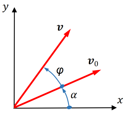
The problem: consider a vector $\boldsymbol v_0$ and rotate it by an angle $\varphi$ around the axis having the direction of the unit vector $\boldsymbol n$ ; the new position of the vector is $\boldsymbol v$ . We have to find the matrix $\boldsymbol R$ , [1], [2], [3], [4]:

\boldsymbol v=\boldsymbol R(\varphi)\boldsymbol v_0.

This is called an active rotation: the vector is rotated while the reference frame remains fixed.

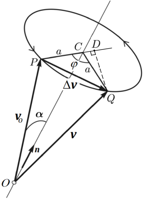
Rotation of vector v0 about the axis n — **Figure 2.** Rotation about the axis $\boldsymbol n$ and the corresponding circular motion.

Displacement of P to Q on the circle of radius a — **Figure 2.** Rotation about the axis $\boldsymbol n$ and the corresponding circular motion.

Vector sum:

\boldsymbol v=\boldsymbol v_0+\Delta\boldsymbol v.

\Delta\boldsymbol v=\overline{PD}+\overline{DQ}\quad\longrightarrow\quad\boldsymbol v=\boldsymbol v_0+\overline{PD}+\overline{DQ}.

Vector $\overline{DQ}$ has the direction of the cross product $\boldsymbol n\times\boldsymbol v_0$ because $\overline{DQ}$ is perpendicular to the plane $(\boldsymbol n,\boldsymbol v_0)$ .

The modulus of $\boldsymbol n\times\boldsymbol v_0$ is:

\lVert\boldsymbol n\times\boldsymbol v_0\rVert=\lVert\boldsymbol v\rVert\sin\alpha\quad\longrightarrow\quad\lVert\boldsymbol n\times\boldsymbol v_0\rVert=a.

As:

DQ=a\sin\varphi,

we get:

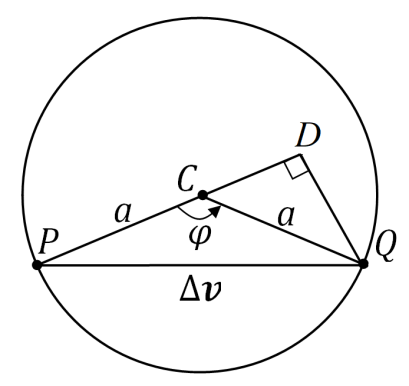
\overline{DQ}=(\boldsymbol n\times\boldsymbol v_0)\sin\varphi.

Vector $\overline{PD}$ . The modulus:

PD=a-a\cos\varphi=2a\sin^2\frac{\varphi}{2}.

Obviously, $\boldsymbol n$ is perpendicular to $\boldsymbol n\times\boldsymbol v_0$ , and thus $\boldsymbol n\times(\boldsymbol n\times\boldsymbol v_0)$ has the direction of vector $\overline{PD}$ . But:

\lVert\boldsymbol n\times(\boldsymbol n\times\boldsymbol v_0)\rVert=\lVert\boldsymbol n\times\boldsymbol v_0\rVert=a,

therefore:

\overline{PD}=2\bigl(\boldsymbol n\times(\boldsymbol n\times\boldsymbol v_0)\bigr)\sin^2\frac{\varphi}{2}.

The relation between $\boldsymbol v$ and $\boldsymbol v_0$ :

\boldsymbol v=\boldsymbol v_0+(\boldsymbol n\times\boldsymbol v_0)\sin\varphi+2\bigl(\boldsymbol n\times(\boldsymbol n\times\boldsymbol v_0)\bigr)\sin^2\frac{\varphi}{2},

or:

\boldsymbol v=\boldsymbol v_0+(\boldsymbol n\times\boldsymbol v_0)\sin\varphi+\bigl(\boldsymbol n\times(\boldsymbol n\times\boldsymbol v_0)\bigr)(1-\cos\varphi).\tag{*}

To convert this equation into matrix form, we introduce the notations:

\boldsymbol n=\begin{Bmatrix}n_x\\n_y\\n_z\end{Bmatrix},\qquad n_x^2+n_y^2+n_z^2=1.

\boldsymbol n\times\boldsymbol v_0\ \longrightarrow\ \begin{bmatrix}0&-n_z&n_y\\n_z&0&-n_x\\-n_y&n_x&0\end{bmatrix}\begin{Bmatrix}v_{0x}\\v_{0y}\\v_{0z}\end{Bmatrix}.

Or:

\boldsymbol n\times\boldsymbol v_0\ \longrightarrow\ \widetilde{\boldsymbol n}\boldsymbol v_0,

with:

\widetilde{\boldsymbol n}=\begin{bmatrix}0&-n_z&n_y\\n_z&0&-n_x\\-n_y&n_x&0\end{bmatrix}.

\boldsymbol n\times(\boldsymbol n\times\boldsymbol v_0)\ \longrightarrow\ \widetilde{\boldsymbol n}^{\,2}\boldsymbol v_0,

where:

\widetilde{\boldsymbol n}^{\,2}=\widetilde{\boldsymbol n}\widetilde{\boldsymbol n}=\begin{bmatrix}-(n_y^2+n_z^2)&n_xn_y&n_zn_x\\n_xn_y&-(n_z^2+n_x^2)&n_yn_z\\n_zn_x&n_yn_z&-(n_x^2+n_y^2)\end{bmatrix}.

This gives:

\boldsymbol v=\bigl(\boldsymbol E+\sin\varphi\,\widetilde{\boldsymbol n}+(1-\cos\varphi)\widetilde{\boldsymbol n}^{\,2}\bigr)\boldsymbol v_0\quad\longrightarrow\quad\boldsymbol v=\boldsymbol R\boldsymbol v_0.

$\boldsymbol E$ is the unit matrix. That is, equation (*) becomes:

\boldsymbol R=\boldsymbol E+\sin\varphi\,\widetilde{\boldsymbol n}+(1-\cos\varphi)\widetilde{\boldsymbol n}^{\,2}.\tag{**}

Finally:

\boldsymbol R=\begin{bmatrix}\cos\varphi+n_x^2(1-\cos\varphi)&n_xn_y(1-\cos\varphi)-n_z\sin\varphi&n_zn_x(1-\cos\varphi)+n_y\sin\varphi\\n_xn_y(1-\cos\varphi)+n_z\sin\varphi&\cos\varphi+n_y^2(1-\cos\varphi)&n_yn_z(1-\cos\varphi)-n_x\sin\varphi\\n_zn_x(1-\cos\varphi)-n_y\sin\varphi&n_yn_z(1-\cos\varphi)+n_x\sin\varphi&\cos\varphi+n_z^2(1-\cos\varphi)\end{bmatrix}.

Another form of the rotation matrix

Now we introduce this vector:

\boldsymbol\rho=\varphi\boldsymbol n=\begin{Bmatrix}\varphi_x\\\varphi_y\\\varphi_z\end{Bmatrix},

and:

\varphi=\sqrt{\varphi_x^2+\varphi_y^2+\varphi_z^2}.

$\boldsymbol\rho$ may be called a rotation vector or axis-angle vector. However, finite rotations do not compose by ordinary vector addition. Relation (**) between $\boldsymbol v$ and $\boldsymbol v_0$ becomes:

\boldsymbol v=\left(\boldsymbol E+\frac{\sin\varphi}{\varphi}\widetilde{\boldsymbol\rho}+\frac{1-\cos\varphi}{\varphi^2}\widetilde{\boldsymbol\rho}^{\,2}\right)\boldsymbol v_0.

And finally:

\begin{aligned}\boldsymbol R={}&\boldsymbol E+\frac{\sin\varphi}{\varphi}\begin{bmatrix}0&-\varphi_z&\varphi_y\\\varphi_z&0&-\varphi_x\\-\varphi_y&\varphi_x&0\end{bmatrix}\\&+\frac{1-\cos\varphi}{\varphi^2}\begin{bmatrix}-(\varphi_y^2+\varphi_z^2)&\varphi_x\varphi_y&\varphi_z\varphi_x\\\varphi_x\varphi_y&-(\varphi_z^2+\varphi_x^2)&\varphi_y\varphi_z\\\varphi_z\varphi_x&\varphi_y\varphi_z&-(\varphi_x^2+\varphi_y^2)\end{bmatrix}.\end{aligned}

Or:

\begin{aligned}\boldsymbol R={}&\boldsymbol E+\sin\varphi\begin{bmatrix}0&-n_z&n_y\\n_z&0&-n_x\\-n_y&n_x&0\end{bmatrix}\\&+(1-\cos\varphi)\begin{bmatrix}-(n_y^2+n_z^2)&n_xn_y&n_zn_x\\n_xn_y&-(n_z^2+n_x^2)&n_yn_z\\n_zn_x&n_yn_z&-(n_x^2+n_y^2)\end{bmatrix}.\end{aligned}

Small rotation angles

If the angle of rotation $\varphi$ is very small:

\frac{\sin\varphi}{\varphi}\approx1.

Neglecting second-degree terms:

\boldsymbol R=\begin{bmatrix}1&-\varphi_z&\varphi_y\\\varphi_z&1&-\varphi_x\\-\varphi_y&\varphi_x&1\end{bmatrix}.

If the rotation angle is small and second-order terms are retained, the rotation angles are assumed to be small, but not infinitesimal; therefore, the second-order terms cannot be neglected. Since the rotation matrix contains quadratic terms in the rotation components, the resulting problem is geometrically nonlinear.

\frac{\sin\varphi}{\varphi}\approx1,\qquad\frac{1-\cos\varphi}{\varphi^2}\approx\frac12.

And:

\boldsymbol R=\begin{bmatrix}1-\frac12(\varphi_y^2+\varphi_z^2)&-\varphi_z+\frac12\varphi_x\varphi_y&\varphi_y+\frac12\varphi_z\varphi_x\\\varphi_z+\frac12\varphi_x\varphi_y&1-\frac12(\varphi_z^2+\varphi_x^2)&-\varphi_x+\frac12\varphi_y\varphi_z\\-\varphi_y+\frac12\varphi_z\varphi_x&\varphi_x+\frac12\varphi_y\varphi_z&1-\frac12(\varphi_x^2+\varphi_y^2)\end{bmatrix}.

Example

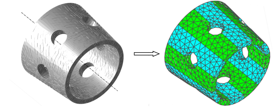
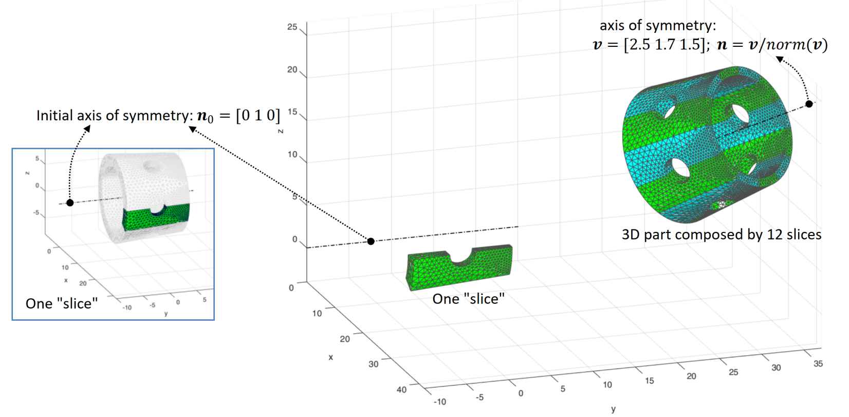
The 3D part in the figure below must be divided into finite elements. The part can be divided into 12 identical slices. Only one slice will be divided into finite elements, and then, by rotating, reflecting and copying this slice, the entire FE mesh will be obtained.

The 3D part and its complete finite element mesh — **Figure 3.** The 3D part and its finite element mesh.

One slice, the axes n0 and n, and the twelve transformed slices — **Figure 4.** One slice and the construction of the complete mesh by rotation and reflection.

One “slice” is depicted in the figure above, on the left. Nodal coordinates are known: $\boldsymbol x$ is a matrix with $n$ rows and 3 columns (for the three coordinates $x,y,z$ ); $n$ is the number of nodes. Coordinates $\boldsymbol x$ are in the global coordinate frame.

Firstly, this slice is rotated around the axis computed using the normalized cross product:

\boldsymbol n_1=\frac{\boldsymbol n_0\times\boldsymbol n}{\lVert\boldsymbol n_0\times\boldsymbol n\rVert},

with the angle computed using a dot product:

\varphi=\arccos(\boldsymbol n_0\cdot\boldsymbol n).

This gives the rotation matrix $\boldsymbol R_1$ :

\boldsymbol R_1=\boldsymbol E+\sin\varphi\,\widetilde{\boldsymbol n}_1+(1-\cos\varphi)\widetilde{\boldsymbol n}_1^{\,2}.

The new coordinates are:

\boldsymbol x_n=\boldsymbol x\boldsymbol R_1^T+\Delta\boldsymbol x,

where $\Delta\boldsymbol x$ contains the translation components, applied to every row. For our example, the translation is $\begin{bmatrix}20&10&5\end{bmatrix}$ .

The remaining slices are obtained with the rotation matrix:

\boldsymbol R_t=\boldsymbol R_2\boldsymbol R_1\quad\longrightarrow\quad\boldsymbol x_n=\boldsymbol x\boldsymbol R_t^T+\Delta\boldsymbol x,

where $\boldsymbol R_2$ is a rotation around the axis defined by the unit vector $\boldsymbol n$ (see the figure above):

\boldsymbol R_2=\boldsymbol E+\sin\varphi_0\,\widetilde{\boldsymbol n}+(1-\cos\varphi_0)\widetilde{\boldsymbol n}^{\,2}.

Angle $\varphi_0$ is a multiple of $\pi/3$ . The 12 slices are obtained at six angular positions spaced by $\pi/3$ , with a reflected and a non-reflected slice at each position. For slices 2, 4, 6, 8, 10 and 12, we need to apply a reflection to obtain the circular holes, with each slice having only a “half-hole”. So the transformation matrix becomes:

\boldsymbol R_t=\boldsymbol R_2\boldsymbol R_1\boldsymbol R_a\quad\longrightarrow\quad\boldsymbol x_n=\boldsymbol x\boldsymbol R_t^T+\Delta\boldsymbol x,

where:

\boldsymbol R_a=\begin{bmatrix}1&0&0\\0&1&0\\0&0&-1\end{bmatrix}.

In fact, the matrix $\boldsymbol R_a$ allows us to build the symmetric slice with respect to the local $xy$ -plane (reflection).

Figure 5. Interactive 3D view of the example. Drag to rotate; switch Zoom ON to use wheel or pinch zoom. Reset view restores the initial camera position.

A simple MATLAB program is available for download below.

MATLABFinite rotations in three dimensionsFour MATLAB files and READMEDownload ZIP ↓

References

[1] Rotation Formula, Wolfram MathWorld.

[2] Finite rotations, Math Wiki.

[3] Carlos Felippa, NFEM, Nonlinear Finite Element Methods (ASEN 5107), Appendix R.

[4] Enrico C. Da Lozzo, Geometrically exact three-dimensional beam theory: modeling and FEM implementation for statics and dynamics analysis, Istituto Universitario di Studi Superiori di Pavia, Master’s Degree in Earthquake Engineering, 2010.