7.2 Beam Structures

Model, hypotheses, and reference frames

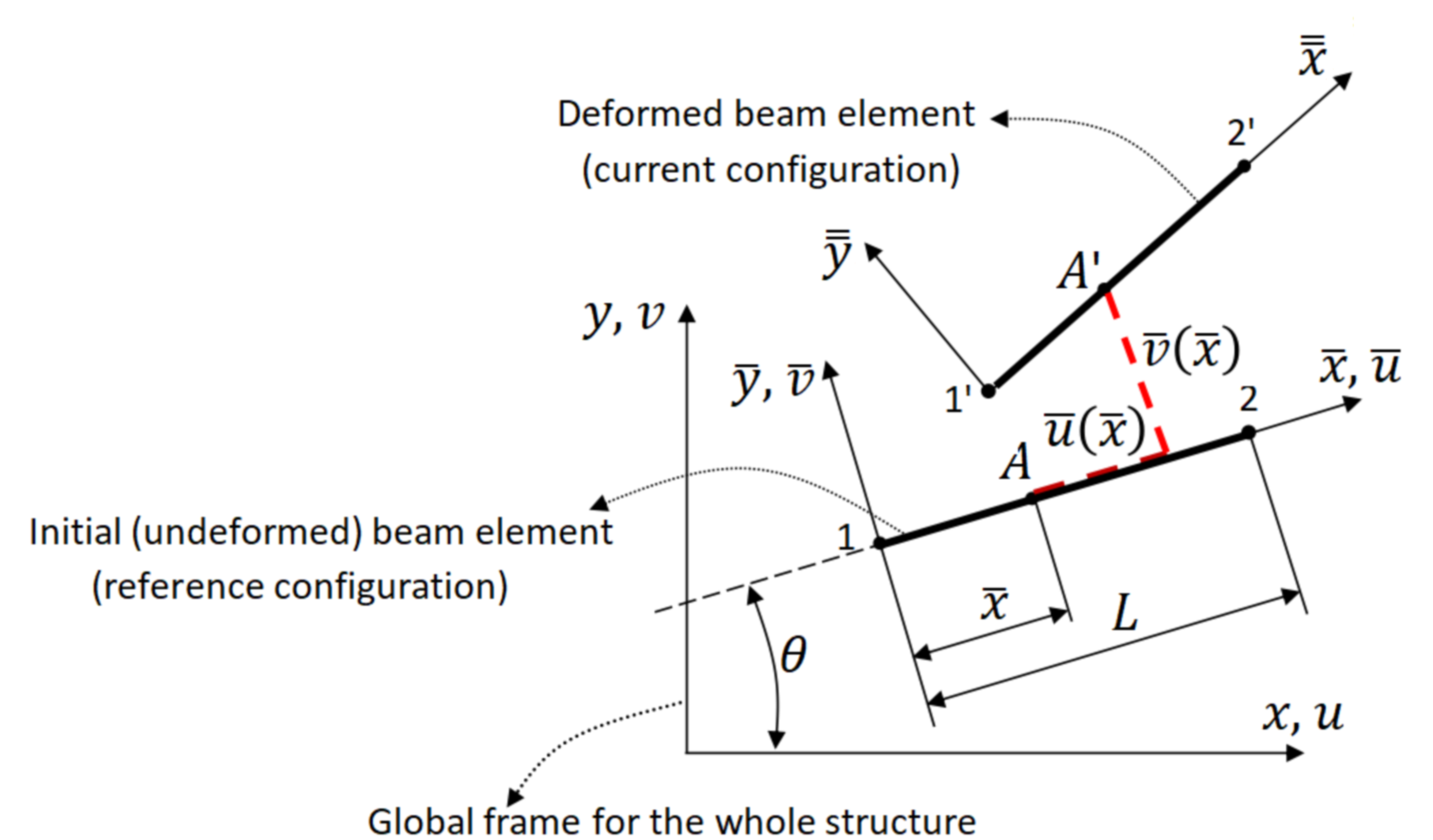
Each beam element has a local reference frame $(\bar{x},\bar{y})$ , whose orientation is fixed with respect to the global frame $(x,y)$ of the structure. Under loading, the structure deforms and each element reaches a new position characterized by the frame $(\bar{\bar{x}},\bar{\bar{y}})$ .

StrainSmall

MaterialLinear elastic

DisplacementLarge

Beam modelTimoshenko

ElementsStraight, prismatic, two-node

ReferenceInitial undeformed configuration

For each beam element, the nodal displacements are expressed in the local reference frame attached to the initial undeformed element. The axial force, shear force, and bending moment are evaluated in this local frame and transformed to the global frame during assembly. Thus, in the Total Lagrangian formulation, both element displacements and internal forces are evaluated with respect to the initial local frame $(\bar{x},\bar{y})$ .

Initial and deformed beam element with global, initial local, and deformed local reference frames — Figure 1. Global structural frame $(x,y)$ , initial local element frame $(\bar{x},\bar{y})$ , and local frame associated with the deformed position $(\bar{\bar{x}},\bar{\bar{y}})$ .

Element transformation

The initial orientation of the undeformed beam element with respect to the global frame is defined by the rotation matrix:

\mathbf R=\begin{bmatrix}\mathbf R_0&\mathbf 0_{3\times3}\\[5pt]\mathbf 0_{3\times3}&\mathbf R_0\end{bmatrix},\qquad \mathbf R_0=\begin{bmatrix}\cos\theta&\sin\theta&0\\[4pt]-\sin\theta&\cos\theta&0\\[4pt]0&0&1\end{bmatrix}

For an element joining nodes 1 and 2,

L=\sqrt{(x_2-x_1)^2+(y_2-y_1)^2},\qquad \cos\theta=\frac{x_2-x_1}{L},\qquad \sin\theta=\frac{y_2-y_1}{L}

The matrix $\mathbf R$ is determined from the initial geometry and remains fixed throughout the Total Lagrangian analysis.

gen.mInitial element rotations

%*** gen ***
Rt = zeros(6,6,nel);
for ie = 1:nel
    n1 = elem(ie,1);
    n2 = elem(ie,2);
    dx = x(n2)-x(n1);
    dy = y(n2)-y(n1);
    L = sqrt(dx*dx+dy*dy);
    cs = dx/L;
    sn = dy/L;
    Lt(ie) = L;
    Rt(:,:,ie) = [ cs sn 0  0  0 0;
                  -sn cs 0  0  0 0;
                    0  0 1  0  0 0;
                    0  0 0 cs sn 0;
                    0  0 0 -sn cs 0;
                    0  0 0  0  0 1];
end

Extension of the element formulation

The formulation developed in Section 7.1 is extended to beam structures with only minor modifications. The programs main.m and deriv.m remain unchanged in their mechanics.

The global element-displacement vector is transformed to the initial local frame before the generalized strains and their derivatives are evaluated:

\boldsymbol u_{el}=\mathbf R\,\boldsymbol U_{el}

stiff.mLocal element displacement

R = Rt(:,:,ie);
s = R*S(ip);

The element internal-force vector and tangent stiffness matrix are transformed back to the global frame during assembly:

\boldsymbol F_{el}=\mathbf R^T\boldsymbol f_{el},\qquad \boldsymbol K_{el}=\mathbf R^T\boldsymbol k_{el}\mathbf R

stiff.mTransformed assembly

F(ip)    = F(ip)    + R'*fel;
K(ip,ip) = K(ip,ip) + R'*kel*R;

Important remark. In the Total Lagrangian formulation presented here, the reference configuration remains the initial undeformed configuration throughout the analysis. Consequently, no incremental approximation associated with the number of load steps is introduced. Within the adopted assumptions, the converged solution is therefore essentially independent of the chosen number of load steps; several load steps may still be useful for tracing the equilibrium path and facilitating convergence.

Example 1 — semicircular beam

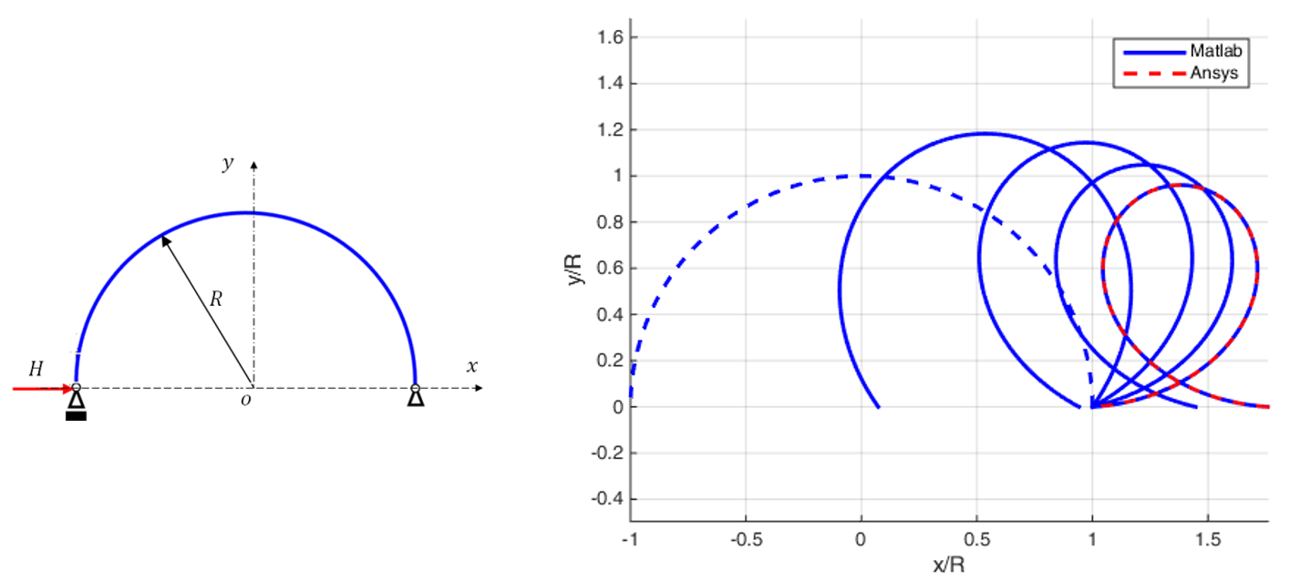
The beam has radius $R=50\ \mathrm{mm}$ , a rectangular cross-section $20\ \mathrm{mm}\times1\ \mathrm{mm}$ (width × thickness), Young's modulus $E=2\times10^5\ \mathrm{MPa}$ , and horizontal load $H=300\ \mathrm N$ .

The figure shows the deformed beam at four equally spaced load levels. For the final load $H=300\ \mathrm N$ , the MATLAB solution is compared with ANSYS, showing very good agreement.

Semicircular beam geometry and deformed configurations compared with ANSYS — Figure 2. Initial geometry, deformed configurations at four equally spaced load levels, and MATLAB–ANSYS comparison at $H=300\ \mathrm N$ .

Internal-force diagrams

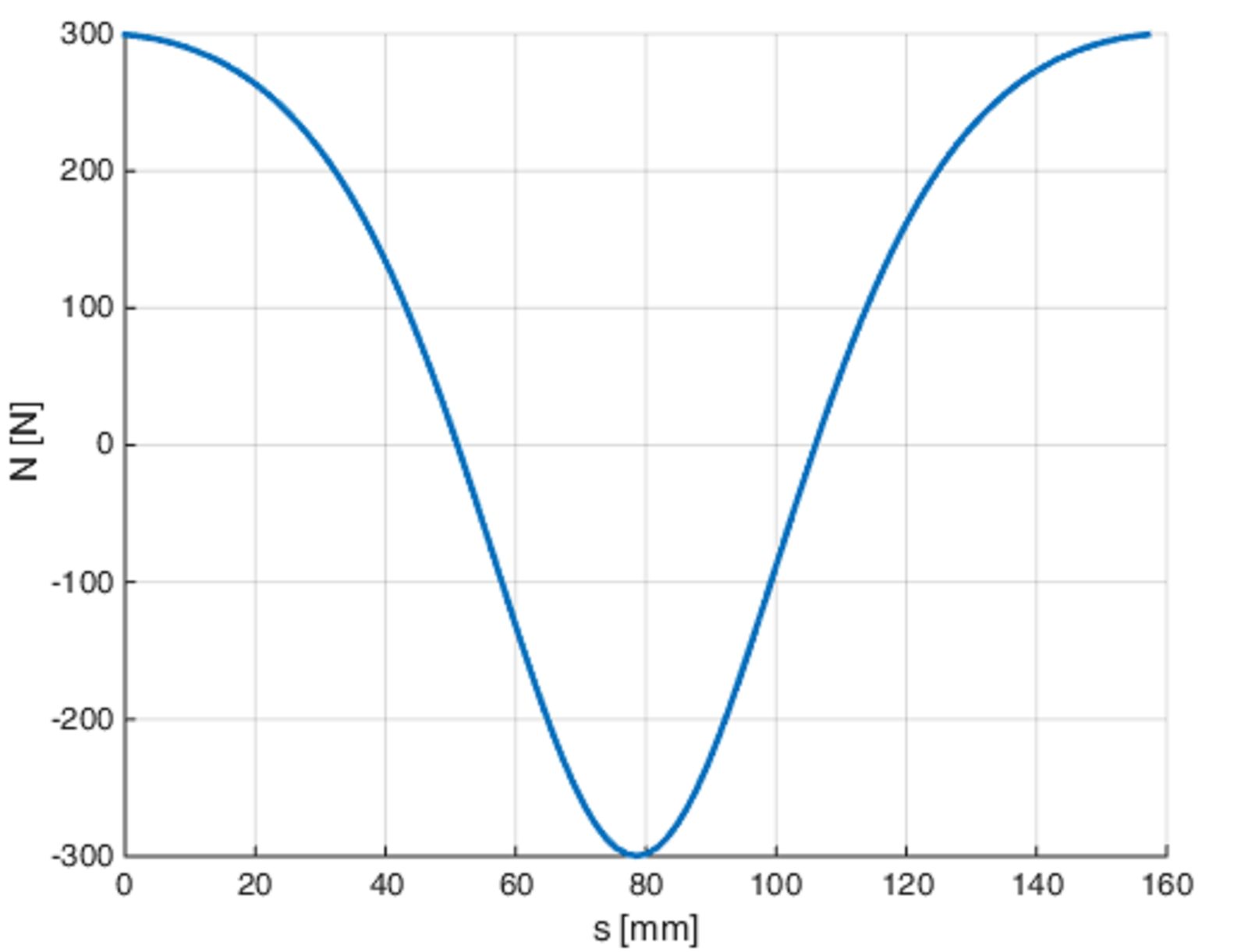
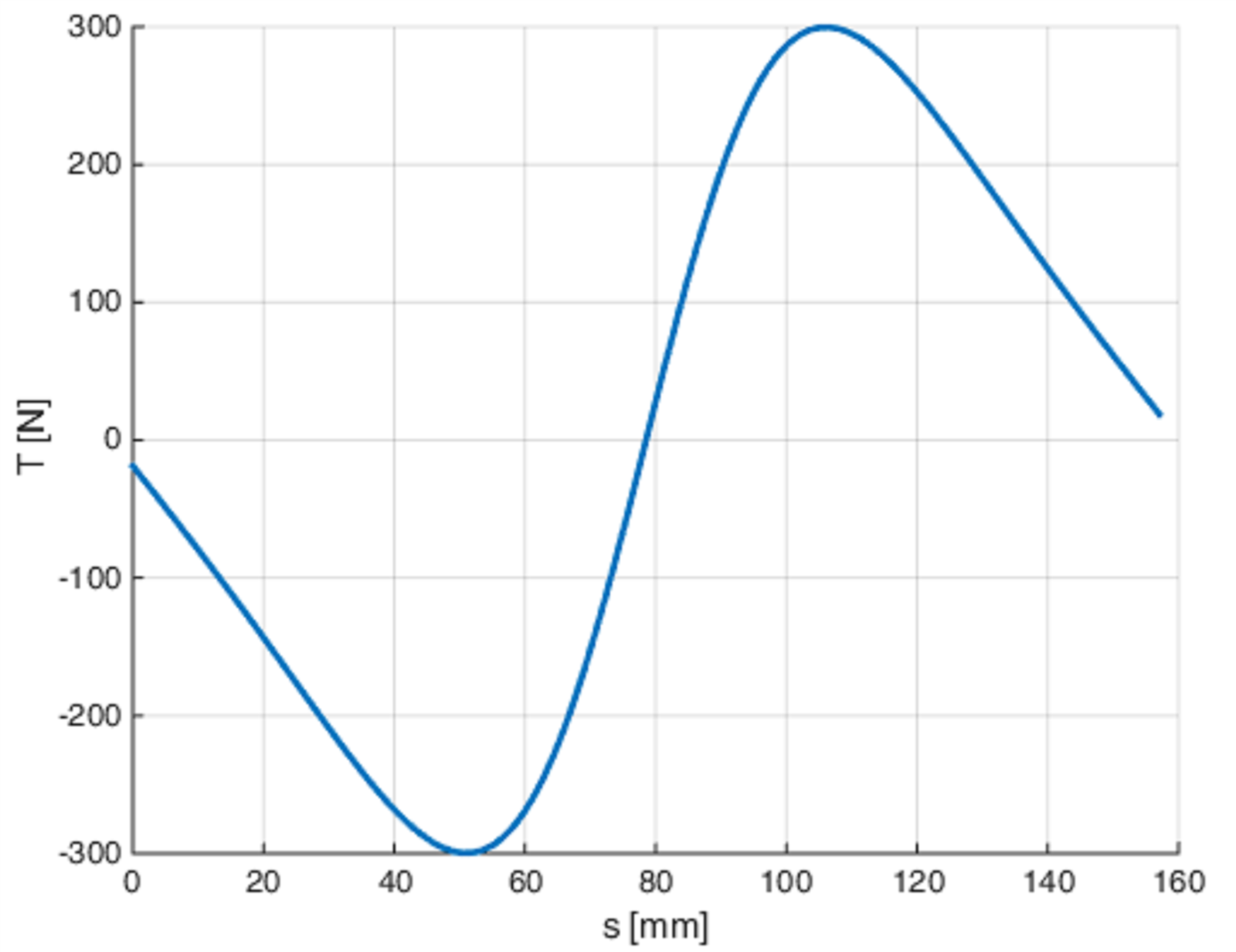
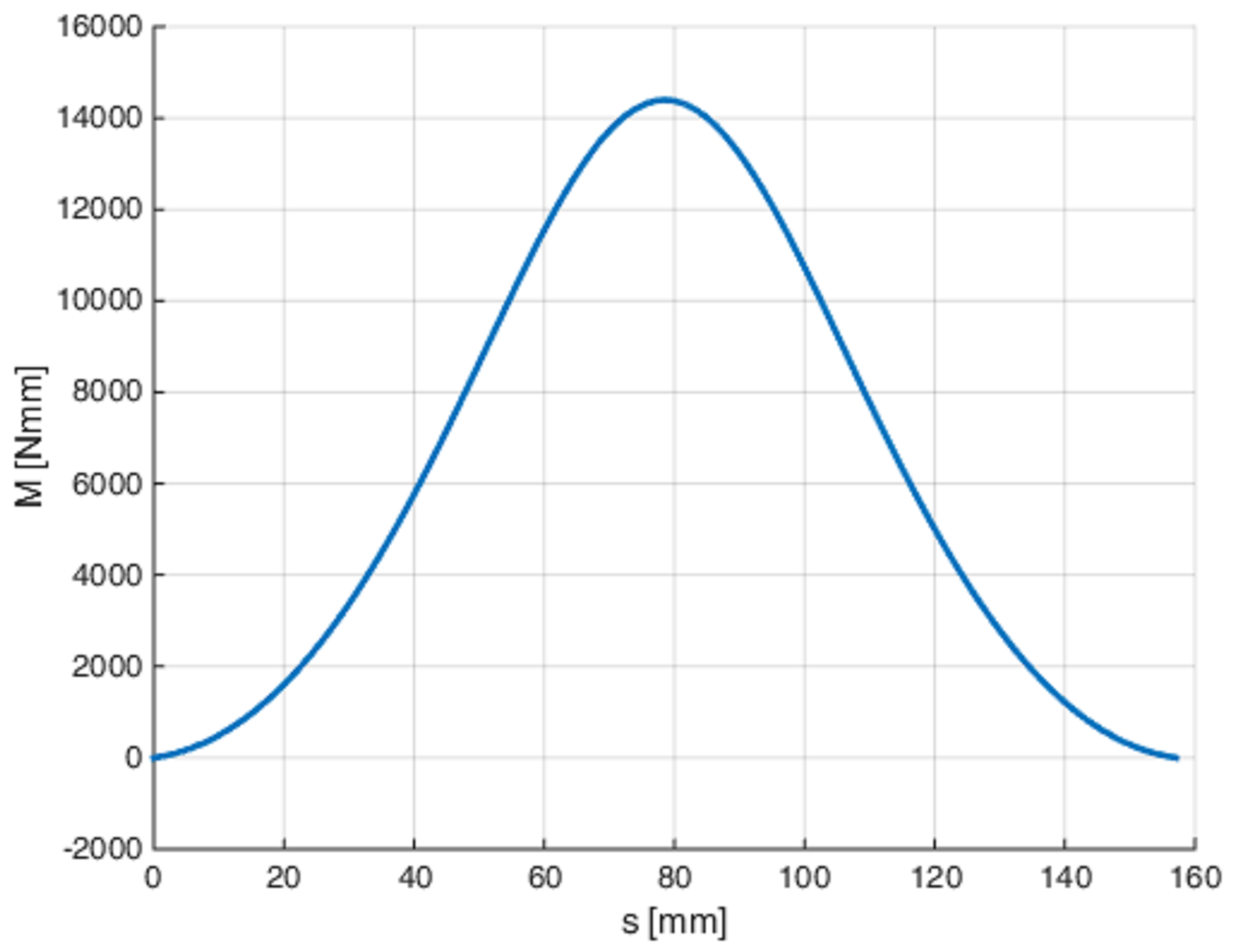
The axial-force, shear-force, and bending-moment diagrams correspond to the final load step. They were plotted using the MATLAB program diagrams.m.

Axial force along the semicircular beam — Figure 3a. Axial force $N$ .

Shear force along the semicircular beam — Figure 3b. Shear force $T$ .

Bending moment along the semicircular beam — Figure 3c. Bending moment $M$ .

Example 2 — Mattiasson benchmark

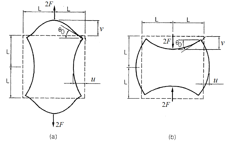
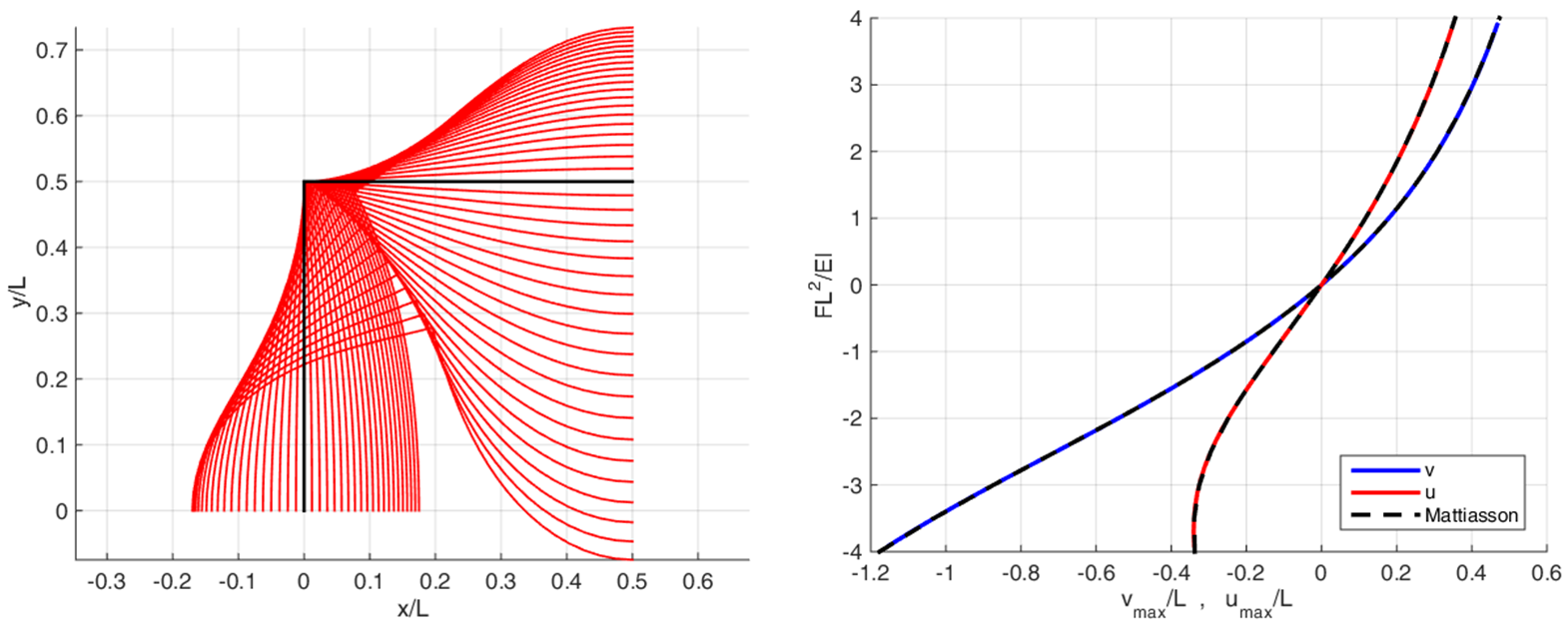
This benchmark is taken from Mattiasson [1], where reference solutions for large-deflection beam and frame problems are obtained using elliptic integrals. The two symmetric loading cases and the displacement components used in the comparison are shown below.

Two large-deflection beam-frame benchmark configurations from Mattiasson — Figure 4. Mattiasson beam-frame benchmark: geometry, loading, and displacement measures $u_{\max}$ and $v_{\max}$ .

The numerical results are compared with the reference solution from [1], and very good agreement is obtained.

Deformed benchmark configurations and normalized response curves compared with Mattiasson — Figure 5. Deformed configurations and normalized load–displacement curves. Solid curves are obtained with the Total Lagrangian beam model; dashed curves are the elliptic-integral reference values from [1].

MATLAB and ANSYS packages

The MATLAB package contains the complete beam-structure analysis, including model generation, local-to-global transformations, nonlinear assembly, result printing, and effort diagrams. The ANSYS package contains the comparison model for Example 1.

MATLAB verification

Tested in MATLAB R2024a. All ten load steps of the distributed example converged in six to eight Newton–Raphson iterations. The code uses standard MATLAB syntax and is expected to be compatible with newer MATLAB versions. No additional toolbox is required.

MTotal Lagrangian beam-structure MATLAB package6 MATLAB files and README · tested in R2024aDownload ZIP AANSYS comparison packageMechanical APDL macro and README · structurally inspected, not executedDownload ZIP

Reference

K. Mattiasson, Numerical results from large deflection beam and frame problems analysed by means of elliptic integrals, International Journal for Numerical Methods in Engineering, 16, 145–153, 1981.