7.1 Cantilever Beam

Model, hypotheses, and notation

The initial, undeformed configuration is used as the reference. The displacement components $u$ and $v$ are measured in the fixed $xy$ frame and may be large, so the equilibrium problem is highly nonlinear.

StrainSmall

MaterialLinear elastic

DisplacementLarge

Beam modelTimoshenko

ElementStraight, prismatic, two-node

ReferenceInitial undeformed configuration

For the Timoshenko beam model in the small-displacement limit,

\left\{\begin{aligned}\kappa&=\frac{d\psi}{dx}=\frac{M}{EI}\\[5pt]\beta&=\frac{T}{GA_0}\\[5pt]\varphi&=\frac{dv}{dx}\\[5pt]\varphi&=\psi+\beta\end{aligned}\right.

\varepsilon_0=\frac{N}{EA}

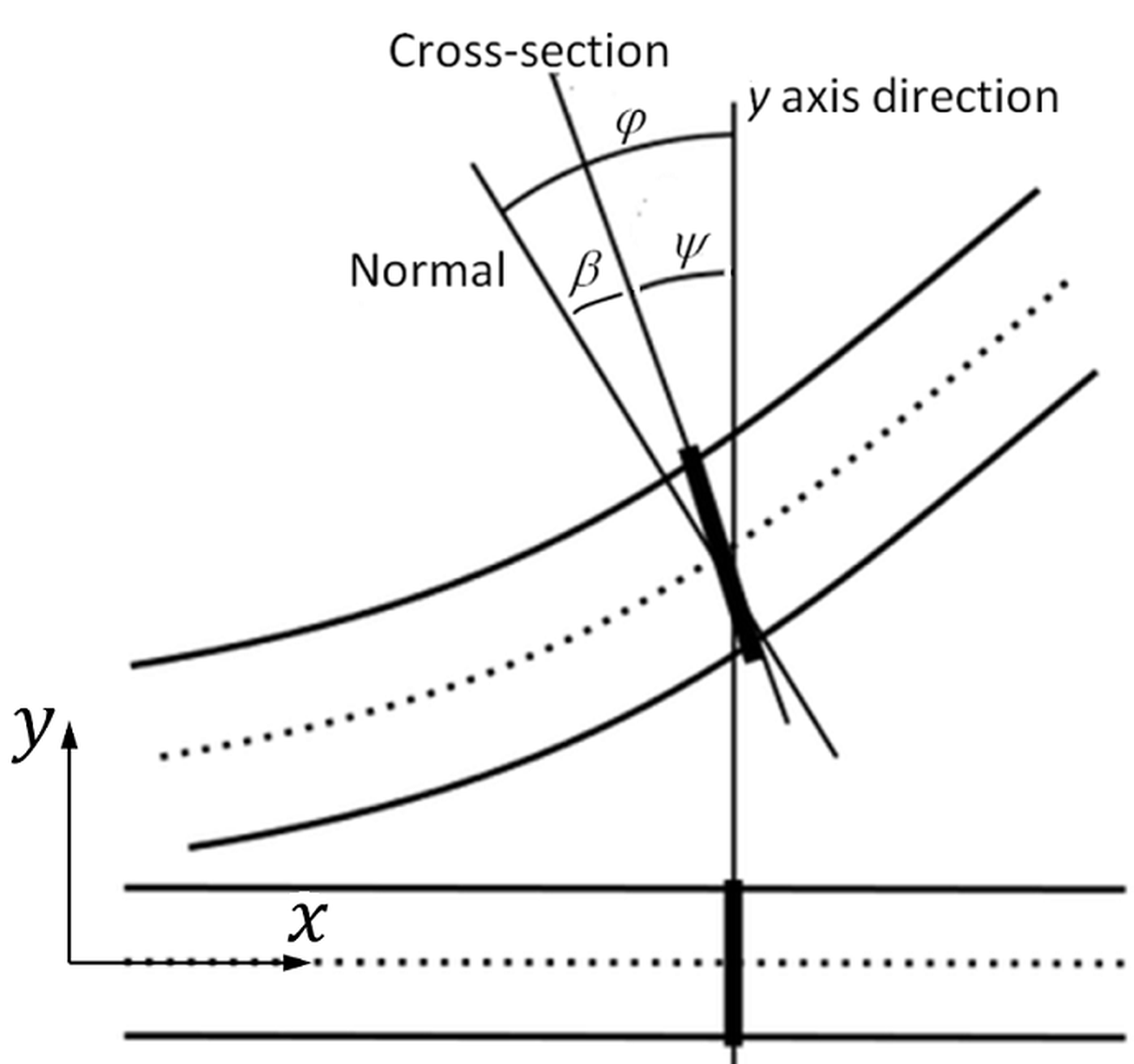
Timoshenko beam kinematics showing the normal, cross-section, and the angles phi, psi, and beta — Figure 1. Timoshenko kinematics: rotation of the normal $\varphi$ , rotation of the cross-section $\psi$ , and shear angle $\beta$ .

As in Sections 5.2 and 5.3, $\beta$ denotes the shear angle, $\varphi$ the rotation of the normal, and $\psi$ the rotation of the cross-section. Thus, the angular nodal degree of freedom of the Timoshenko beam element is $\psi$ , not $\varphi$ .

\beta=\varphi-\psi

For the Timoshenko beam model, the angular nodal degree of freedom is $\psi$ , not $\varphi$ . The same distinction is used in Sections 5.2 and 5.3.

$N,T,M$: axial force, shear force, and bending moment
$E,G$: Young's modulus and shear modulus
$A,A_0,I$: cross-sectional area, shear area, and second moment of area
$u,v$: displacements along the initial $x$ and $y$ axes

Exact kinematics and generalized strains

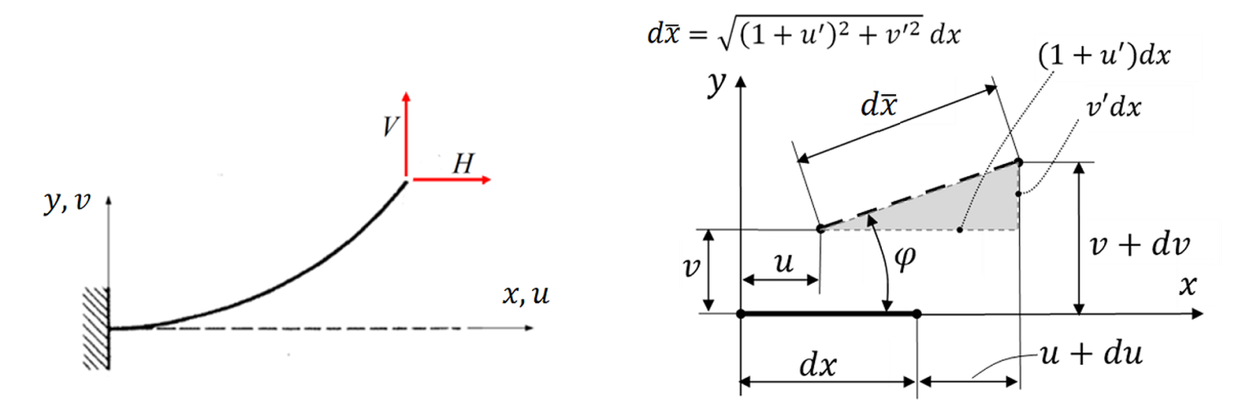
Cantilever loads and differential geometry of the deformed neutral axis — Figure 2. Cantilever loading and differential geometry used to define the rotation and axial strain.

From the geometry shown above, the rotation of the normal is:

\tan\varphi=\frac{v'}{1+u'}

All derivatives in this formulation are taken with respect to the axial coordinate $x$ of the initial configuration:

u'=\frac{du}{dx},\qquad v'=\frac{dv}{dx}

The generalized strain vector is:

\boldsymbol{\varepsilon}=\begin{Bmatrix}\varepsilon_0\\[5pt]\beta\\[5pt]\kappa\end{Bmatrix}

Pythagoras' theorem applied to the differential neutral-axis segment gives:

d\bar{x}=\sqrt{(1+u')^2+v'^2}\,dx

and therefore the exact axial strain of the neutral axis is:

\varepsilon_0=\frac{d\bar{x}}{dx}-1=\sqrt{(1+u')^2+v'^2}-1

The curvature and shear angle are:

\kappa=\frac{d\psi}{dx}

\beta=\operatorname{atan}\!\left(\frac{v'}{1+u'}\right)-\psi

Isoparametric interpolation

A two-node isoparametric beam element is adopted. To avoid using the same symbol for arc length and the beam natural coordinate, the natural coordinate is denoted by $\xi\in[-1,1]$ .

x(\xi)=h_1(\xi)x_1+h_2(\xi)x_2,\qquad y(\xi)=h_1(\xi)y_1+h_2(\xi)y_2

h_1(\xi)=\frac{1-\xi}{2},\qquad h_2(\xi)=\frac{1+\xi}{2}

The same linear functions interpolate the displacement components and cross-section rotation:

\left\{\begin{aligned}u(\xi)&=h_1(\xi)u_1+h_2(\xi)u_2\\[4pt]v(\xi)&=h_1(\xi)v_1+h_2(\xi)v_2\\[4pt]\psi(\xi)&=h_1(\xi)\psi_1+h_2(\xi)\psi_2\end{aligned}\right.

For a straight element with $x_2>x_1$ ,

\frac{d\xi}{dx}=\left(\frac{dx}{d\xi}\right)^{-1}=\left(\frac{x_2-x_1}{2}\right)^{-1}=\frac{2}{L}

The exact element strains are then

\varepsilon_0=\sqrt{\left(1+\frac{u_2-u_1}{L}\right)^2+\left(\frac{v_2-v_1}{L}\right)^2}-1

L=\sqrt{(x_2-x_1)^2+(y_2-y_1)^2}=x_2-x_1\qquad(y_1=y_2=0)

\kappa=\frac{\psi_2-\psi_1}{L}

\beta(\xi)=\operatorname{atan}\!\left(\frac{v_2-v_1}{L+u_2-u_1}\right)-\left(\frac{1-\xi}{2}\psi_1+\frac{1+\xi}{2}\psi_2\right)

At the one-point Gauss location $\xi=0$ ,

\beta_0=\beta(0)=\operatorname{atan}\!\left(\frac{v_2-v_1}{L+u_2-u_1}\right)-\frac{\psi_1+\psi_2}{2}

Deformation energy and element equations

The deformation energy of one finite element is:

U_{el}=\frac12\int_0^L\left(EA\varepsilon_0^2+GA_0\beta^2+EI\kappa^2\right)dx

With one Gauss point at $\xi=0$ ,

U_{el}=\frac{L}{2}\left(EA\varepsilon_0^2+GA_0\beta_0^2+EI\kappa^2\right)

The element nodal-displacement vector is:

\boldsymbol u_{el}=\begin{Bmatrix}u_1\\[4pt]v_1\\[4pt]\psi_1\\[4pt]u_2\\[4pt]v_2\\[4pt]\psi_2\end{Bmatrix}

The element internal-force vector and tangent stiffness matrix follow from the first and second derivatives of the energy:

\boldsymbol f_{el}=\frac{\partial U_{el}}{\partial\boldsymbol u_{el}},\qquad \boldsymbol k_{el}=\frac{\partial\boldsymbol f_{el}}{\partial\boldsymbol u_{el}}=\frac{\partial^2U_{el}}{\partial\boldsymbol u_{el}^2}

\boldsymbol f_{el}=L\left(EA\varepsilon_0\frac{\partial\varepsilon_0}{\partial\boldsymbol u_{el}}+GA_0\beta_0\frac{\partial\beta_0}{\partial\boldsymbol u_{el}}+EI\kappa\frac{\partial\kappa}{\partial\boldsymbol u_{el}}\right)

\boldsymbol k_{el}=L\left[EA\varepsilon_0\frac{\partial^2\varepsilon_0}{\partial\boldsymbol u_{el}^2}+EA\frac{\partial\varepsilon_0}{\partial\boldsymbol u_{el}}\left(\frac{\partial\varepsilon_0}{\partial\boldsymbol u_{el}}\right)^T+GA_0\beta_0\frac{\partial^2\beta_0}{\partial\boldsymbol u_{el}^2}+GA_0\frac{\partial\beta_0}{\partial\boldsymbol u_{el}}\left(\frac{\partial\beta_0}{\partial\boldsymbol u_{el}}\right)^T+EI\kappa\frac{\partial^2\kappa}{\partial\boldsymbol u_{el}^2}+EI\frac{\partial\kappa}{\partial\boldsymbol u_{el}}\left(\frac{\partial\kappa}{\partial\boldsymbol u_{el}}\right)^T\right]

Strain derivatives and the length approximation

Introduce the exact deformed element length

L_f=\sqrt{(L+u_2-u_1)^2+(v_2-v_1)^2}

The first derivatives used in the element residual are:

\frac{\partial\varepsilon_0}{\partial\boldsymbol u_{el}}=\frac{1}{LL_f}\begin{Bmatrix}-L+u_1-u_2\\[4pt]v_1-v_2\\[4pt]0\\[4pt]L-u_1+u_2\\[4pt]-v_1+v_2\\[4pt]0\end{Bmatrix}

\frac{\partial\beta_0}{\partial\boldsymbol u_{el}}=\frac{1}{L_f^2}\begin{Bmatrix}-v_1+v_2\\[4pt]-L+u_1-u_2\\[4pt]-L_f^2/2\\[4pt]v_1-v_2\\[4pt]L-u_1+u_2\\[4pt]-L_f^2/2\end{Bmatrix}

\frac{\partial\kappa}{\partial\boldsymbol u_{el}}=\frac1L\begin{Bmatrix}0\\[3pt]0\\[3pt]-1\\[3pt]0\\[3pt]0\\[3pt]1\end{Bmatrix},\qquad \frac{\partial^2\kappa}{\partial\boldsymbol u_{el}^2}=\boldsymbol0_{6\times6}

The derivatives of $L_f$ are neglected when evaluating the following second-order derivatives.

\frac{\partial^2\varepsilon_0}{\partial\boldsymbol u_{el}^2}\cong\frac{1}{LL_f}\begin{bmatrix}1&0&0&-1&0&0\\[4pt]0&1&0&0&-1&0\\[4pt]0&0&0&0&0&0\\[4pt]-1&0&0&1&0&0\\[4pt]0&-1&0&0&1&0\\[4pt]0&0&0&0&0&0\end{bmatrix}

\frac{\partial^2\beta_0}{\partial\boldsymbol u_{el}^2}\cong\frac{1}{L_f^2}\begin{bmatrix}0&-1&0&0&1&0\\[4pt]1&0&0&-1&0&0\\[4pt]0&0&0&0&0&0\\[4pt]0&1&0&0&-1&0\\[4pt]-1&0&0&1&0&0\\[4pt]0&0&0&0&0&0\end{bmatrix}

The exact relation between the deformed and initial element lengths is retained before the small-strain simplification:

L_f=(1+\varepsilon_0)L

Because the axial strain is very small,

\varepsilon_0\ll1

and therefore:

L_f=(1+\varepsilon_0)L\approx L

The derivative expressions used in the program become

\frac{\partial\varepsilon_0}{\partial\boldsymbol u_{el}}=\frac{1}{L^2}\begin{Bmatrix}-L+u_1-u_2\\[4pt]v_1-v_2\\[4pt]0\\[4pt]L-u_1+u_2\\[4pt]-v_1+v_2\\[4pt]0\end{Bmatrix}

\frac{\partial^2\varepsilon_0}{\partial\boldsymbol u_{el}^2}=\frac{1}{L^2}\begin{bmatrix}1&0&0&-1&0&0\\[4pt]0&1&0&0&-1&0\\[4pt]0&0&0&0&0&0\\[4pt]-1&0&0&1&0&0\\[4pt]0&-1&0&0&1&0\\[4pt]0&0&0&0&0&0\end{bmatrix}

\frac{\partial\beta_0}{\partial\boldsymbol u_{el}}=\frac{1}{L^2}\begin{Bmatrix}-v_1+v_2\\[4pt]-L+u_1-u_2\\[4pt]-L^2/2\\[4pt]v_1-v_2\\[4pt]L-u_1+u_2\\[4pt]-L^2/2\end{Bmatrix}

\frac{\partial^2\beta_0}{\partial\boldsymbol u_{el}^2}=\frac{1}{L^2}\begin{bmatrix}0&-1&0&0&1&0\\[4pt]1&0&0&-1&0&0\\[4pt]0&0&0&0&0&0\\[4pt]0&1&0&0&-1&0\\[4pt]-1&0&0&1&0&0\\[4pt]0&0&0&0&0&0\end{bmatrix}

Nonlinear equilibrium and solution

The assembled residual vector and tangent stiffness matrix are:

\boldsymbol\Psi=\sum_{el}\boldsymbol f_{el}-\boldsymbol F,\qquad \boldsymbol K_t=\sum_{el}\boldsymbol k_{el}

Equivalently, with total potential energy $\Pi=U-\boldsymbol u^T\boldsymbol F$ ,

\boldsymbol\Psi=\frac{\partial\Pi}{\partial\boldsymbol u}=\frac{\partial U}{\partial\boldsymbol u}-\boldsymbol F=\boldsymbol0

The Newton–Raphson iteration is:

\Delta\boldsymbol u^{(i)}=-\left[\boldsymbol K_t\!\left(\boldsymbol u^{(i)}\right)\right]^{-1}\boldsymbol\Psi\!\left(\boldsymbol u^{(i)}\right)

\boldsymbol u^{(i+1)}=\boldsymbol u^{(i)}+\Delta\boldsymbol u^{(i)}

main.mNewton–Raphson loop

%*** main ***
error = 1;
iter = 0;
while (error > tol) && (iter < itermax)
    iter = iter + 1;
    stiff
    dS = K\F;
    S = S - dS;
    error = sqrt(dS'*dS/nnd);
end

The iteration is stopped when the displacement-correction norm is smaller than the prescribed tolerance. Four to eight iterations are usually sufficient for the examples considered.

Important remark. Within the adopted assumptions, the presented Total Lagrangian formulation does not introduce an incremental approximation associated with the number of load steps. Consequently, the solution error is not controlled by the number of load increments in the same way as in an incremental approximation; a single load step may be sufficient even for very large displacements.

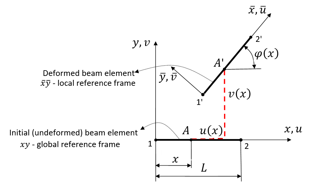
Initial and deformed two-node beam element in the Total Lagrangian description — Figure 3. Total Lagrangian description: $u(x)$ and $v(x)$ are defined on the initial element $x\in[0,L]$ .

Numerical examples

Both examples use $L=100\ \mathrm{mm}$ , a rectangular cross-section $5\ \mathrm{mm}\times1\ \mathrm{mm}$ (width × thickness), and $E=2\times10^5\ \mathrm{MPa}$ . The finite-element results are compared with the elliptic-integral values tabulated by Mattiasson [1].

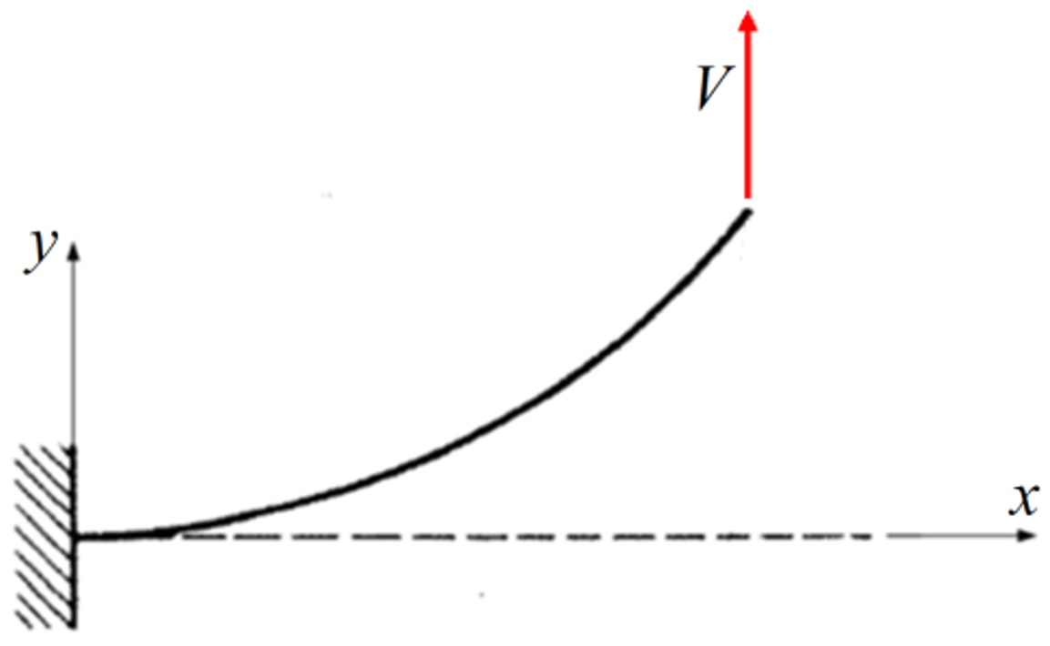
Cantilever under a vertical free-end force V — Figure 4. Cantilever and positive transverse free-end force $V$ .

Example a. The cantilever is loaded by $V=100\ \mathrm N$ and $H=0$ .

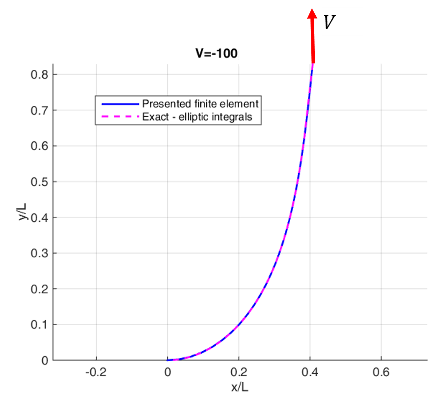
Deformed cantilever under V equals 100 newtons compared with the elliptic-integral solution — Figure 5. Deformed cantilever for $V=100\ \mathrm N$ . The Total Lagrangian and elliptic-integral curves coincide visually.

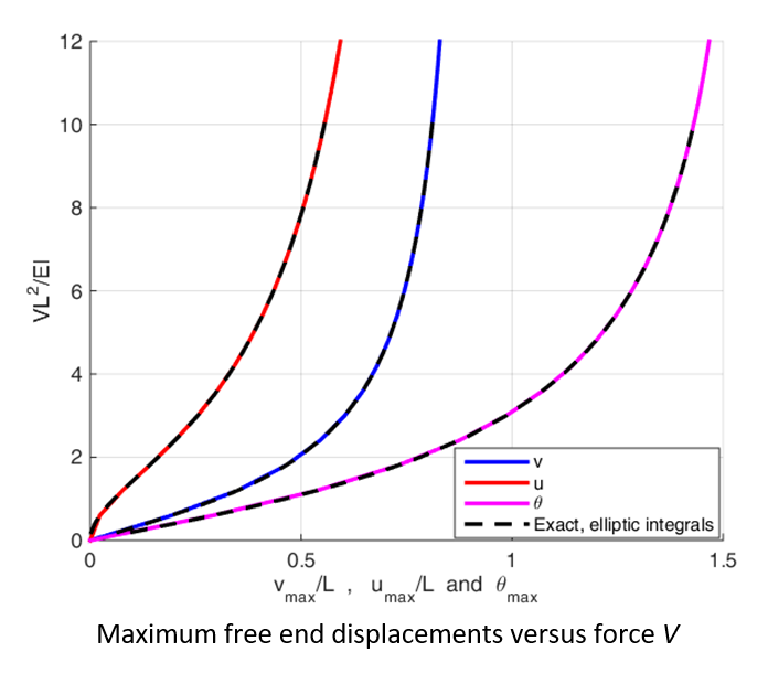
Maximum free-end displacement and rotation versus vertical force — Figure 6. Maximum free-end axial displacement, transverse displacement, and rotation versus $V$ .

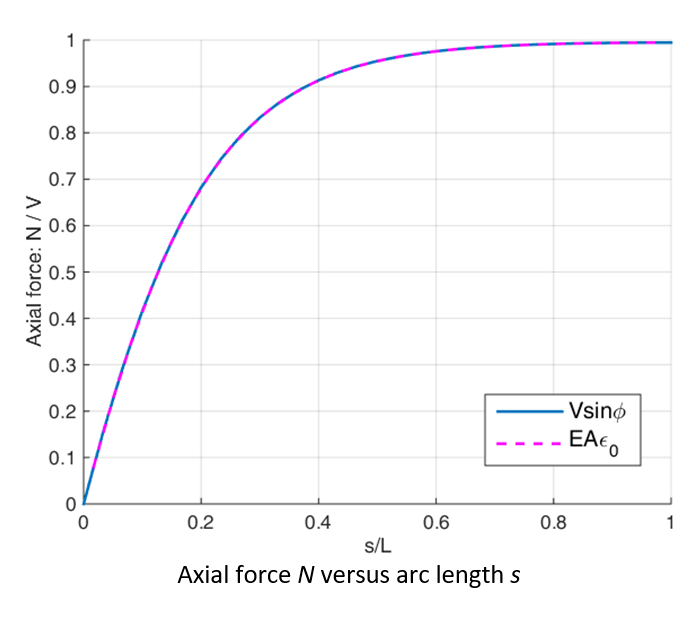
Axial force versus arc length for the transversely loaded cantilever — Figure 7. Axial force along the deformed-beam arc length $s$ . The equality $N=EA\varepsilon_0$ agrees with the force component $V\sin\varphi$ .

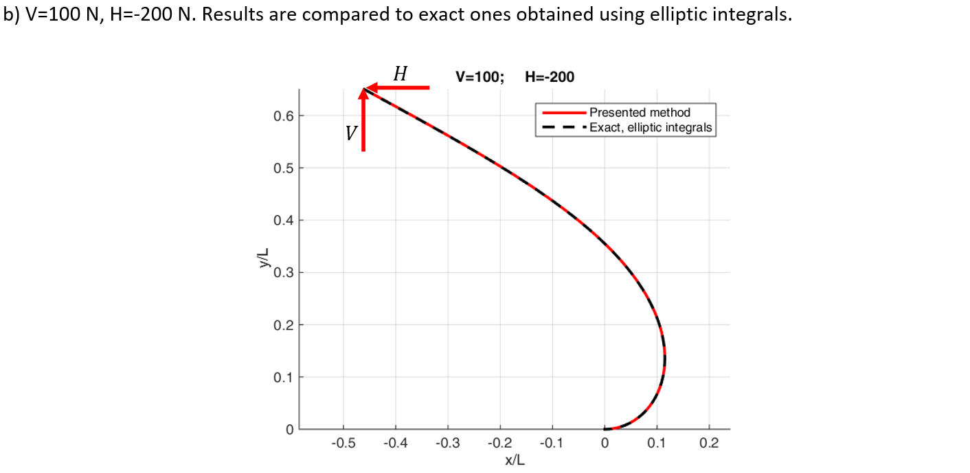
Example b. The cantilever is loaded by $V=100\ \mathrm N$ and $H=-200\ \mathrm N$ .

Deformed cantilever under vertical and horizontal free-end forces compared with the elliptic-integral solution — Figure 8. Deformed cantilever under the combined free-end forces. The presented and elliptic-integral solutions coincide visually.

The elliptic-integral beam solution does not include the Timoshenko shear contribution. That contribution is included in the present formulation and is usually small for the slender beam used in these examples.

MATLAB programs

The package contains the complete Total Lagrangian analysis. deriv.m evaluates the generalized strains and derivatives; stiff.m forms and assembles the internal-force vector and tangent matrix; main.m performs load stepping and Newton–Raphson iterations; and the remaining files define the model, print results, and draw effort diagrams.

MATLAB compatibility

Prepared for MATLAB R2024a. The code uses standard MATLAB syntax and is expected to be compatible with R2024a and newer MATLAB versions. No additional toolbox is required.

MTotal Lagrangian cantilever MATLAB package6 commented MATLAB files and README · prepared for R2024aDownload ZIP

Reference

K. Mattiasson, Numerical results from large deflection beam and frame problems analysed by means of elliptic integrals, International Journal for Numerical Methods in Engineering, 17(1), 145–153, 1981.