Hypotheses:
Strain Small
Displacement Small
Material Linear
Euler–Bernoulli beam model.
Beam element: straight, prismatic (constant cross-section), two nodes.
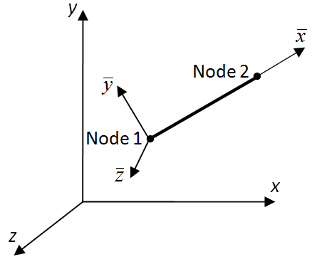
The local reference frame is composed of the beam centroidal axis, the local x ˉ \bar x x ˉ y ˉ \bar y y ˉ z ˉ \bar z z ˉ ( u , v , w ) (u,v,w) ( u , v , w ) ( φ x , φ y , φ z ) (\varphi_x,\varphi_y,\varphi_z) ( φ x , φ y , φ z )
Figure 1. In the local reference frame:
u ‾ e l = { u ˉ 1 v ˉ 1 w ˉ 1 φ x ˉ 1 φ y ˉ 1 φ z ˉ 1 u ˉ 2 v ˉ 2 w ˉ 2 φ x ˉ 2 φ y ˉ 2 φ z ˉ 2 } T .
\overline{\boldsymbol{u}}_{el}=
\left\{
\begin{array}{cccccccccccc}
\bar u_1&
\bar v_1&
\bar w_1&
\varphi_{\bar x1}&
\varphi_{\bar y1}&
\varphi_{\bar z1}&
\bar u_2&
\bar v_2&
\bar w_2&
\varphi_{\bar x2}&
\varphi_{\bar y2}&
\varphi_{\bar z2}
\end{array}
\right\}^{T}.
u e l = { u ˉ 1 v ˉ 1 w ˉ 1 φ x ˉ 1 φ y ˉ 1 φ z ˉ 1 u ˉ 2 v ˉ 2 w ˉ 2 φ x ˉ 2 φ y ˉ 2 φ z ˉ 2 } T . In the global reference frame:
u e l = { u 1 v 1 w 1 φ x 1 φ y 1 φ z 1 u 2 v 2 w 2 φ x 2 φ y 2 φ z 2 } T .
\boldsymbol{u}_{el}=
\left\{
\begin{array}{cccccccccccc}
u_1&
v_1&
w_1&
\varphi_{x1}&
\varphi_{y1}&
\varphi_{z1}&
u_2&
v_2&
w_2&
\varphi_{x2}&
\varphi_{y2}&
\varphi_{z2}
\end{array}
\right\}^{T}.
u e l = { u 1 v 1 w 1 φ x 1 φ y 1 φ z 1 u 2 v 2 w 2 φ x 2 φ y 2 φ z 2 } T . 01 Notations used for the beam elementHooke’s law:
σ = D ε ,
\boldsymbol{\sigma}=\boldsymbol{D}\boldsymbol{\varepsilon},
σ = D ε , or
{ N M x ˉ M y ˉ M z ˉ } = [ E A 0 0 0 0 G I t 0 0 0 0 E I y 0 0 0 0 E I z ] { ε 0 κ x ˉ κ y ˉ κ z ˉ } .
\left\{
\begin{array}{c}
N\\
M_{\bar x}\\
M_{\bar y}\\
M_{\bar z}
\end{array}
\right\}
=
\begin{bmatrix}
EA&0&0&0\\
0&GI_t&0&0\\
0&0&EI_y&0\\
0&0&0&EI_z
\end{bmatrix}
\left\{
\begin{array}{c}
\varepsilon_0\\
\kappa_{\bar x}\\
\kappa_{\bar y}\\
\kappa_{\bar z}
\end{array}
\right\}.
⎩ ⎨ ⎧ N M x ˉ M y ˉ M z ˉ ⎭ ⎬ ⎫ = E A 0 0 0 0 G I t 0 0 0 0 E I y 0 0 0 0 E I z ⎩ ⎨ ⎧ ε 0 κ x ˉ κ y ˉ κ z ˉ ⎭ ⎬ ⎫ . The generalized strain and stress vectors are
ε = { ε 0 κ x ˉ κ y ˉ κ z ˉ } , σ = { N M x ˉ M y ˉ M z ˉ } .
\boldsymbol{\varepsilon}=
\left\{
\begin{array}{c}
\varepsilon_0\\
\kappa_{\bar x}\\
\kappa_{\bar y}\\
\kappa_{\bar z}
\end{array}
\right\},
\qquad
\boldsymbol{\sigma}=
\left\{
\begin{array}{c}
N\\
M_{\bar x}\\
M_{\bar y}\\
M_{\bar z}
\end{array}
\right\}.
ε = ⎩ ⎨ ⎧ ε 0 κ x ˉ κ y ˉ κ z ˉ ⎭ ⎬ ⎫ , σ = ⎩ ⎨ ⎧ N M x ˉ M y ˉ M z ˉ ⎭ ⎬ ⎫ . The constitutive matrix is
D = [ E A 0 0 0 0 G I t 0 0 0 0 E I y 0 0 0 0 E I z ] .
\boldsymbol{D}=
\begin{bmatrix}
EA&0&0&0\\
0&GI_t&0&0\\
0&0&EI_y&0\\
0&0&0&EI_z
\end{bmatrix}.
D = E A 0 0 0 0 G I t 0 0 0 0 E I y 0 0 0 0 E I z . The axial strain of the centroidal axis is
ε 0 = d u ˉ d x ˉ .
\varepsilon_0=\frac{d\bar u}{d\bar x}.
ε 0 = d x ˉ d u ˉ . In the Euler–Bernoulli beam model, the slopes in the two principal planes are
φ y ˉ = − d w ˉ d x ˉ , φ z ˉ = d v ˉ d x ˉ .
\varphi_{\bar y}=-\frac{d\bar w}{d\bar x},
\qquad
\varphi_{\bar z}=\frac{d\bar v}{d\bar x}.
φ y ˉ = − d x ˉ d w ˉ , φ z ˉ = d x ˉ d v ˉ . Consequently,
κ x ˉ = d φ x ˉ d x ˉ ,
\kappa_{\bar x}=
\frac{d\varphi_{\bar x}}{d\bar x},
κ x ˉ = d x ˉ d φ x ˉ , κ y ˉ = d φ y ˉ d x ˉ = − d 2 w ˉ d x ˉ 2 ,
\kappa_{\bar y}=
\frac{d\varphi_{\bar y}}{d\bar x}
=
-\frac{d^2\bar w}{d\bar x^2},
κ y ˉ = d x ˉ d φ y ˉ = − d x ˉ 2 d 2 w ˉ , κ z ˉ = d φ z ˉ d x ˉ = d 2 v ˉ d x ˉ 2 .
\kappa_{\bar z}=
\frac{d\varphi_{\bar z}}{d\bar x}
=
\frac{d^2\bar v}{d\bar x^2}.
κ z ˉ = d x ˉ d φ z ˉ = d x ˉ 2 d 2 v ˉ . Thus the sign associated with bending about the local y ˉ \bar y y ˉ κ y ˉ \kappa_{\bar y} κ y ˉ
M x ˉ = G I t κ x ˉ , M y ˉ = E I y κ y ˉ , M z ˉ = E I z κ z ˉ .
M_{\bar x}=GI_t\kappa_{\bar x},
\qquad
M_{\bar y}=EI_y\kappa_{\bar y},
\qquad
M_{\bar z}=EI_z\kappa_{\bar z}.
M x ˉ = G I t κ x ˉ , M y ˉ = E I y κ y ˉ , M z ˉ = E I z κ z ˉ . N N N M x ˉ M_{\bar x} M x ˉ M y ˉ , M z ˉ M_{\bar y},M_{\bar z} M y ˉ , M z ˉ
E E E G G G
A , I t , I y , I z A,I_t,I_y,I_z A , I t , I y , I z
02 Interpolation functions in the local reference frameThe deflected centroidal axis of the beam is described by a third-degree polynomial for the two transverse displacements v ˉ \bar v v ˉ w ˉ \bar w w ˉ u ˉ \bar u u ˉ φ x ˉ \varphi_{\bar x} φ x ˉ
In the Euler–Bernoulli beam model, in the local reference frame, the slopes are [1] :
φ y ˉ = − d w ˉ d x ˉ , φ z ˉ = d v ˉ d x ˉ .
\varphi_{\bar y}=-\frac{d\bar w}{d\bar x},
\qquad
\varphi_{\bar z}=\frac{d\bar v}{d\bar x}.
φ y ˉ = − d x ˉ d w ˉ , φ z ˉ = d x ˉ d v ˉ . Consequently, the six displacement components have the following variation along the beam element.
Let
ξ = x ˉ L ,
\xi=\frac{\bar x}{L},
ξ = L x ˉ , where L L L
Axial displacement — linear polynomial
u ˉ ( ξ ) = ( 1 − ξ ) u ˉ 1 + ξ u ˉ 2 .
\bar u(\xi)
=
(1-\xi)\bar u_1+\xi\bar u_2.
u ˉ ( ξ ) = ( 1 − ξ ) u ˉ 1 + ξ u ˉ 2 . Twist angle — linear polynomial
φ x ˉ ( ξ ) = ( 1 − ξ ) φ x ˉ 1 + ξ φ x ˉ 2 .
\varphi_{\bar x}(\xi)
=
(1-\xi)\varphi_{\bar x1}
+
\xi\varphi_{\bar x2}.
φ x ˉ ( ξ ) = ( 1 − ξ ) φ x ˉ 1 + ξ φ x ˉ 2 . Transverse displacement and slope in the x ˉ y ˉ \bar x\bar y x ˉ y ˉ
Define:
H 1 = 2 ξ 3 − 3 ξ 2 + 1 ,
H_1=2\xi^3-3\xi^2+1,
H 1 = 2 ξ 3 − 3 ξ 2 + 1 , H 2 = L ( ξ 3 − 2 ξ 2 + ξ ) ,
H_2=L(\xi^3-2\xi^2+\xi),
H 2 = L ( ξ 3 − 2 ξ 2 + ξ ) , H 3 = − 2 ξ 3 + 3 ξ 2 ,
H_3=-2\xi^3+3\xi^2,
H 3 = − 2 ξ 3 + 3 ξ 2 , H 4 = L ( ξ 3 − ξ 2 ) .
H_4=L(\xi^3-\xi^2).
H 4 = L ( ξ 3 − ξ 2 ) . Then
v ˉ = H 1 v ˉ 1 + H 2 φ z ˉ 1 + H 3 v ˉ 2 + H 4 φ z ˉ 2 ,
\bar v
=
H_1\bar v_1
+
H_2\varphi_{\bar z1}
+
H_3\bar v_2
+
H_4\varphi_{\bar z2},
v ˉ = H 1 v ˉ 1 + H 2 φ z ˉ 1 + H 3 v ˉ 2 + H 4 φ z ˉ 2 , and
φ z ˉ = d v ˉ d x ˉ .
\varphi_{\bar z}=\frac{d\bar v}{d\bar x}.
φ z ˉ = d x ˉ d v ˉ . Transverse displacement and slope in the x ˉ z ˉ \bar x\bar z x ˉ z ˉ
w ˉ = H 1 w ˉ 1 − H 2 φ y ˉ 1 + H 3 w ˉ 2 − H 4 φ y ˉ 2 ,
\bar w
=
H_1\bar w_1
-
H_2\varphi_{\bar y1}
+
H_3\bar w_2
-
H_4\varphi_{\bar y2},
w ˉ = H 1 w ˉ 1 − H 2 φ y ˉ 1 + H 3 w ˉ 2 − H 4 φ y ˉ 2 , and
φ y ˉ = − d w ˉ d x ˉ .
\varphi_{\bar y}=-\frac{d\bar w}{d\bar x}.
φ y ˉ = − d x ˉ d w ˉ . Hence,
u ‾ ( x ˉ ) = N ( x ˉ ) u ‾ e l ,
\overline{\boldsymbol{u}}(\bar x)
=
\boldsymbol{N}(\bar x)\,
\overline{\boldsymbol{u}}_{el},
u ( x ˉ ) = N ( x ˉ ) u e l , where
u ‾ ( x ˉ ) = { u ˉ v ˉ w ˉ φ x ˉ φ y ˉ φ z ˉ } .
\overline{\boldsymbol{u}}(\bar x)
=
\left\{
\begin{array}{c}
\bar u\\
\bar v\\
\bar w\\
\varphi_{\bar x}\\
\varphi_{\bar y}\\
\varphi_{\bar z}
\end{array}
\right\}.
u ( x ˉ ) = ⎩ ⎨ ⎧ u ˉ v ˉ w ˉ φ x ˉ φ y ˉ φ z ˉ ⎭ ⎬ ⎫ . The interpolation functions satisfy exactly the Euler–Bernoulli kinematic assumptions.
It results the matrix B \boldsymbol{B} B [1] :
ε = { ε 0 κ x ˉ κ y ˉ κ z ˉ } = { d u ˉ d x ˉ d φ x ˉ d x ˉ − d 2 w ˉ d x ˉ 2 d 2 v ˉ d x ˉ 2 } = B u ‾ e l ,
\boldsymbol{\varepsilon}
=
\left\{
\begin{array}{c}
\varepsilon_0\\
\kappa_{\bar x}\\
\kappa_{\bar y}\\
\kappa_{\bar z}
\end{array}
\right\}
=
\left\{
\begin{array}{c}
\dfrac{d\bar u}{d\bar x}\\[2mm]
\dfrac{d\varphi_{\bar x}}{d\bar x}\\[2mm]
-\dfrac{d^2\bar w}{d\bar x^2}\\[2mm]
\dfrac{d^2\bar v}{d\bar x^2}
\end{array}
\right\}
=
\boldsymbol{B}\,
\overline{\boldsymbol{u}}_{el},
ε = ⎩ ⎨ ⎧ ε 0 κ x ˉ κ y ˉ κ z ˉ ⎭ ⎬ ⎫ = ⎩ ⎨ ⎧ d x ˉ d u ˉ d x ˉ d φ x ˉ − d x ˉ 2 d 2 w ˉ d x ˉ 2 d 2 v ˉ ⎭ ⎬ ⎫ = B u e l , that is,
B = [ − 1 L 0 0 0 0 0 1 L 0 0 0 0 0 0 0 0 − 1 L 0 0 0 0 0 1 L 0 0 0 0 6 − 12 ξ L 2 0 − 4 + 6 ξ L 0 0 0 − 6 + 12 ξ L 2 0 − 2 + 6 ξ L 0 0 − 6 + 12 ξ L 2 0 0 0 − 4 + 6 ξ L 0 6 − 12 ξ L 2 0 0 0 − 2 + 6 ξ L ] .
\boldsymbol{B}=
\begin{bmatrix}
-\dfrac1L&0&0&0&0&0&
\dfrac1L&0&0&0&0&0
\\[3mm]
0&0&0&-\dfrac1L&0&0&
0&0&0&\dfrac1L&0&0
\\[3mm]
0&0&\dfrac{6-12\xi}{L^2}&0&
\dfrac{-4+6\xi}{L}&0&
0&0&\dfrac{-6+12\xi}{L^2}&0&
\dfrac{-2+6\xi}{L}&0
\\[3mm]
0&\dfrac{-6+12\xi}{L^2}&0&0&0&
\dfrac{-4+6\xi}{L}&
0&\dfrac{6-12\xi}{L^2}&0&0&0&
\dfrac{-2+6\xi}{L}
\end{bmatrix}.
B = − L 1 0 0 0 0 0 0 L 2 − 6 + 12 ξ 0 0 L 2 6 − 12 ξ 0 0 − L 1 0 0 0 0 L − 4 + 6 ξ 0 0 0 0 L − 4 + 6 ξ L 1 0 0 0 0 0 0 L 2 6 − 12 ξ 0 0 L 2 − 6 + 12 ξ 0 0 L 1 0 0 0 0 L − 2 + 6 ξ 0 0 0 0 L − 2 + 6 ξ . 03 Element stiffness matrixThe deformation energy for a single finite element is
U e l = 1 2 ∫ L ε T σ d x ˉ ,
U_{el}=
\frac12
\int_L
\boldsymbol{\varepsilon}^{T}
\boldsymbol{\sigma}\,
d\bar x,
U e l = 2 1 ∫ L ε T σ d x ˉ , or
U e l = 1 2 ∫ L ε T D ε d x ˉ .
U_{el}=
\frac12
\int_L
\boldsymbol{\varepsilon}^{T}
\boldsymbol{D}
\boldsymbol{\varepsilon}\,
d\bar x.
U e l = 2 1 ∫ L ε T D ε d x ˉ . Using
ε = B u ‾ e l ,
\boldsymbol{\varepsilon}
=
\boldsymbol{B}\overline{\boldsymbol{u}}_{el},
ε = B u e l , we obtain
U e l = 1 2 u ‾ e l T [ ∫ L B T D B d x ˉ ] u ‾ e l = 1 2 u ‾ e l T k ‾ e l u ‾ e l ,
U_{el}
=
\frac12
\overline{\boldsymbol{u}}_{el}^{\,T}
\left[
\int_L
\boldsymbol{B}^T\boldsymbol{D}\boldsymbol{B}\,d\bar x
\right]
\overline{\boldsymbol{u}}_{el}
=
\frac12
\overline{\boldsymbol{u}}_{el}^{\,T}
\overline{\boldsymbol{k}}_{el}
\overline{\boldsymbol{u}}_{el},
U e l = 2 1 u e l T [ ∫ L B T D B d x ˉ ] u e l = 2 1 u e l T k e l u e l , where
k ‾ e l = ∫ L B T D B d x ˉ .
\boxed{
\overline{\boldsymbol{k}}_{el}
=
\int_L
\boldsymbol{B}^T\boldsymbol{D}\boldsymbol{B}\,d\bar x
}.
k e l = ∫ L B T D B d x ˉ . The integral can be calculated analytically. It results:
k ‾ e l = [ E A L 0 0 0 0 0 − E A L 0 0 0 0 0 0 12 E I z L 3 0 0 0 6 E I z L 2 0 − 12 E I z L 3 0 0 0 6 E I z L 2 0 0 12 E I y L 3 0 − 6 E I y L 2 0 0 0 − 12 E I y L 3 0 − 6 E I y L 2 0 0 0 0 G I t L 0 0 0 0 0 − G I t L 0 0 0 0 − 6 E I y L 2 0 4 E I y L 0 0 0 6 E I y L 2 0 2 E I y L 0 0 6 E I z L 2 0 0 0 4 E I z L 0 − 6 E I z L 2 0 0 0 2 E I z L − E A L 0 0 0 0 0 E A L 0 0 0 0 0 0 − 12 E I z L 3 0 0 0 − 6 E I z L 2 0 12 E I z L 3 0 0 0 − 6 E I z L 2 0 0 − 12 E I y L 3 0 6 E I y L 2 0 0 0 12 E I y L 3 0 6 E I y L 2 0 0 0 0 − G I t L 0 0 0 0 0 G I t L 0 0 0 0 − 6 E I y L 2 0 2 E I y L 0 0 0 6 E I y L 2 0 4 E I y L 0 0 6 E I z L 2 0 0 0 2 E I z L 0 − 6 E I z L 2 0 0 0 4 E I z L ] .
\overline{\boldsymbol{k}}_{el}=
\begin{bmatrix}
\frac{EA}{L}&0&0&0&0&0&-\frac{EA}{L}&0&0&0&0&0\\
0&\frac{12EI_z}{L^3}&0&0&0&\frac{6EI_z}{L^2}&0&-\frac{12EI_z}{L^3}&0&0&0&\frac{6EI_z}{L^2}\\
0&0&\frac{12EI_y}{L^3}&0&-\frac{6EI_y}{L^2}&0&0&0&-\frac{12EI_y}{L^3}&0&-\frac{6EI_y}{L^2}&0\\
0&0&0&\frac{GI_t}{L}&0&0&0&0&0&-\frac{GI_t}{L}&0&0\\
0&0&-\frac{6EI_y}{L^2}&0&\frac{4EI_y}{L}&0&0&0&\frac{6EI_y}{L^2}&0&\frac{2EI_y}{L}&0\\
0&\frac{6EI_z}{L^2}&0&0&0&\frac{4EI_z}{L}&0&-\frac{6EI_z}{L^2}&0&0&0&\frac{2EI_z}{L}\\
-\frac{EA}{L}&0&0&0&0&0&\frac{EA}{L}&0&0&0&0&0\\
0&-\frac{12EI_z}{L^3}&0&0&0&-\frac{6EI_z}{L^2}&0&\frac{12EI_z}{L^3}&0&0&0&-\frac{6EI_z}{L^2}\\
0&0&-\frac{12EI_y}{L^3}&0&\frac{6EI_y}{L^2}&0&0&0&\frac{12EI_y}{L^3}&0&\frac{6EI_y}{L^2}&0\\
0&0&0&-\frac{GI_t}{L}&0&0&0&0&0&\frac{GI_t}{L}&0&0\\
0&0&-\frac{6EI_y}{L^2}&0&\frac{2EI_y}{L}&0&0&0&\frac{6EI_y}{L^2}&0&\frac{4EI_y}{L}&0\\
0&\frac{6EI_z}{L^2}&0&0&0&\frac{2EI_z}{L}&0&-\frac{6EI_z}{L^2}&0&0&0&\frac{4EI_z}{L}
\end{bmatrix}.
k e l = L E A 0 0 0 0 0 − L E A 0 0 0 0 0 0 L 3 12 E I z 0 0 0 L 2 6 E I z 0 − L 3 12 E I z 0 0 0 L 2 6 E I z 0 0 L 3 12 E I y 0 − L 2 6 E I y 0 0 0 − L 3 12 E I y 0 − L 2 6 E I y 0 0 0 0 L G I t 0 0 0 0 0 − L G I t 0 0 0 0 − L 2 6 E I y 0 L 4 E I y 0 0 0 L 2 6 E I y 0 L 2 E I y 0 0 L 2 6 E I z 0 0 0 L 4 E I z 0 − L 2 6 E I z 0 0 0 L 2 E I z − L E A 0 0 0 0 0 L E A 0 0 0 0 0 0 − L 3 12 E I z 0 0 0 − L 2 6 E I z 0 L 3 12 E I z 0 0 0 − L 2 6 E I z 0 0 − L 3 12 E I y 0 L 2 6 E I y 0 0 0 L 3 12 E I y 0 L 2 6 E I y 0 0 0 0 − L G I t 0 0 0 0 0 L G I t 0 0 0 0 − L 2 6 E I y 0 L 2 E I y 0 0 0 L 2 6 E I y 0 L 4 E I y 0 0 L 2 6 E I z 0 0 0 L 2 E I z 0 − L 2 6 E I z 0 0 0 L 4 E I z . 04 Transformation from the global to the local reference frameTo transform the displacement components from the global reference frame to the local reference frame, the passive rotation matrix R \boldsymbol{R} R
u ‾ e l = R u e l .
\boxed{
\overline{\boldsymbol{u}}_{el}
=
\boldsymbol{R}\,\boldsymbol{u}_{el}
}.
u e l = R u e l . The element rotation matrix is
R = [ R 0 0 0 0 0 R 0 0 0 0 0 R 0 0 0 0 0 R 0 ] ,
\boldsymbol{R}=
\begin{bmatrix}
\boldsymbol{R}_0&\boldsymbol{0}&\boldsymbol{0}&\boldsymbol{0}\\
\boldsymbol{0}&\boldsymbol{R}_0&\boldsymbol{0}&\boldsymbol{0}\\
\boldsymbol{0}&\boldsymbol{0}&\boldsymbol{R}_0&\boldsymbol{0}\\
\boldsymbol{0}&\boldsymbol{0}&\boldsymbol{0}&\boldsymbol{R}_0
\end{bmatrix},
R = R 0 0 0 0 0 R 0 0 0 0 0 R 0 0 0 0 0 R 0 , where
R 0 = [ l 1 m 1 n 1 l 2 m 2 n 2 l 3 m 3 n 3 ] .
\boldsymbol{R}_0=
\begin{bmatrix}
l_1&m_1&n_1\\
l_2&m_2&n_2\\
l_3&m_3&n_3
\end{bmatrix}.
R 0 = l 1 l 2 l 3 m 1 m 2 m 3 n 1 n 2 n 3 . Matrix R 0 \boldsymbol{R}_0 R 0 R 0 \boldsymbol{R}_0 R 0
Therefore,
U e l = 1 2 u e l T R T k ‾ e l R u e l = 1 2 u e l T k e l u e l ,
U_{el}
=
\frac12
\boldsymbol{u}_{el}^T
\boldsymbol{R}^T
\overline{\boldsymbol{k}}_{el}
\boldsymbol{R}
\boldsymbol{u}_{el}
=
\frac12
\boldsymbol{u}_{el}^T
\boldsymbol{k}_{el}
\boldsymbol{u}_{el},
U e l = 2 1 u e l T R T k e l R u e l = 2 1 u e l T k e l u e l , and hence
k e l = R T k ‾ e l R .
\boxed{
\boldsymbol{k}_{el}
=
\boldsymbol{R}^T
\overline{\boldsymbol{k}}_{el}
\boldsymbol{R}
}.
k e l = R T k e l R . This is the same passive transformation convention used for finite-element assembly throughout the 3D developments.
05 Definition of the local reference frameThe simplest way to define the direction of the local reference frame for each beam element is to attach a third node n 3 n_3 n 3 n 1 n_1 n 1 n 2 n_2 n 2
The plane defined by the three nodes n 1 , n 2 , n 3 n_1,n_2,n_3 n 1 , n 2 , n 3 x ˉ y ˉ \bar x\bar y x ˉ y ˉ
The third node n 3 n_3 n 3 n 1 n_1 n 1 n 2 n_2 n 2
A MATLAB computer code is available for download.
MATLAB 3D beam element — Euler–Bernoulli model Download ZIP Subprogram princ, called by gen, computes the 3 × 3 3\times3 3 × 3 R 0 \boldsymbol{R}_0 R 0
06 Numerical integrationAlthough the integral
∫ L B T D B d x ˉ
\int_L
\boldsymbol{B}^T\boldsymbol{D}\boldsymbol{B}\,d\bar x
∫ L B T D B d x ˉ can be calculated analytically, in the MATLAB subprogram beam3d we prefer to compute it using the Gauss method with two integration points.
The result is exact because B \boldsymbol{B} B x ˉ \bar x x ˉ
B T D B
\boldsymbol{B}^T\boldsymbol{D}\boldsymbol{B}
B T D B contains polynomials of at most second degree.
This approach is very convenient for nonlinear problems, for instance problems with large displacements.
Therefore,
∫ L B T D B d x ˉ = L 2 [ B ( x ˉ G 1 ) T D B ( x ˉ G 1 ) + B ( x ˉ G 2 ) T D B ( x ˉ G 2 ) ] ,
\int_L
\boldsymbol{B}^T\boldsymbol{D}\boldsymbol{B}\,d\bar x
=
\frac L2
\left[
\boldsymbol{B}(\bar x_{G1})^T
\boldsymbol{D}
\boldsymbol{B}(\bar x_{G1})
+
\boldsymbol{B}(\bar x_{G2})^T
\boldsymbol{D}
\boldsymbol{B}(\bar x_{G2})
\right],
∫ L B T D B d x ˉ = 2 L [ B ( x ˉ G 1 ) T D B ( x ˉ G 1 ) + B ( x ˉ G 2 ) T D B ( x ˉ G 2 ) ] , where x ˉ G 1 \bar x_{G1} x ˉ G 1 x ˉ G 2 \bar x_{G2} x ˉ G 2
x ˉ G 1 = L 2 ( 1 − 3 3 ) ,
\bar x_{G1}
=
\frac L2
\left(
1-\frac{\sqrt3}{3}
\right),
x ˉ G 1 = 2 L ( 1 − 3 3 ) , and
x ˉ G 2 = L 2 ( 1 + 3 3 ) .
\bar x_{G2}
=
\frac L2
\left(
1+\frac{\sqrt3}{3}
\right).
x ˉ G 2 = 2 L ( 1 + 3 3 ) . The origin of the local x ˉ \bar x x ˉ
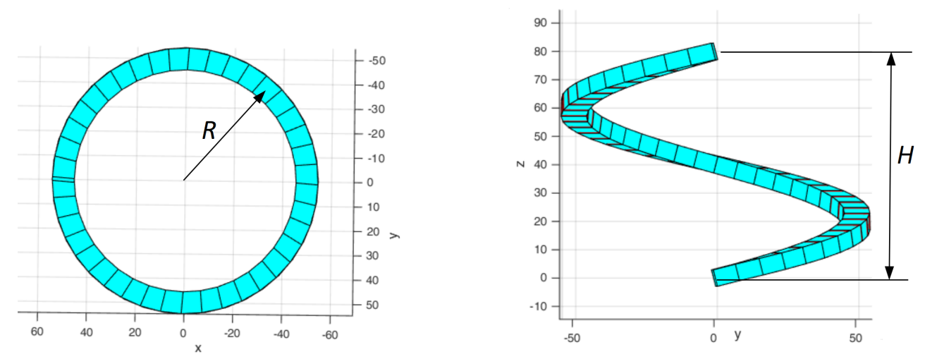
07 ExampleA clamped, curved helicoidal beam is analysed:
R = 50 m m , H = 80 m m ,
R=50\ {\rm mm},
\qquad
H=80\ {\rm mm},
R = 50 mm , H = 80 mm , with a rectangular cross-section
h × b = 9 × 6 m m .
h\times b=9\times6\ {\rm mm}.
h × b = 9 × 6 mm . Refer to the MATLAB subprogram gen for all input data.
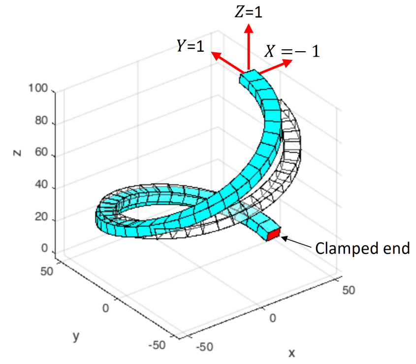
Figure 2. The undeformed and deformed shapes of the beam are shown in the figure below; the displacement scale is 1.
Figure 3. PREVIOUS SECTION ← 22.2. 3D cantilever beam with large displacements. Finite difference method NEXT SECTION 23.2. 3D beam element. Timoshenko model →