23.2. 3D beam element. Timoshenko model

Hypotheses:

StrainSmall

DisplacementSmall

MaterialLinear

Timoshenko beam model.

Beam element: straight, prismatic (constant cross-section), two nodes.

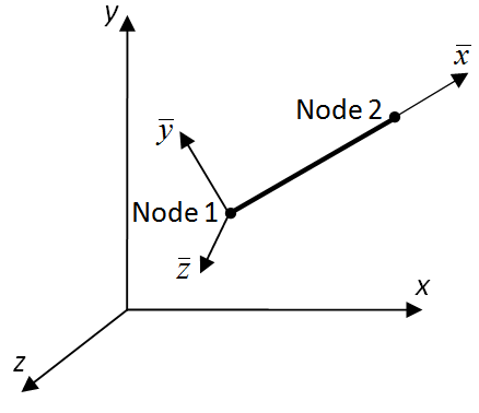
The local reference frame contains the beam centroidal axis, the local $\bar x$ -axis, and the two principal axes of the constant cross-section, the local $\bar y$ - and $\bar z$ -axes. Each node has six DOFs.

In the local reference frame, these DOFs are three displacements

(\bar u,\bar v,\bar w)

and three rotations of the cross-section

(\psi_{\bar x},\psi_{\bar y},\psi_{\bar z}).

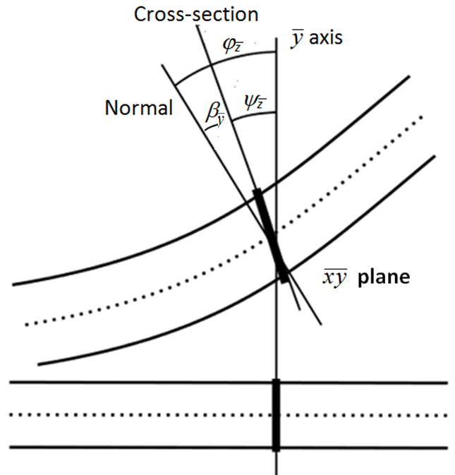
For the Timoshenko beam, the nodal rotations are the rotations of the cross-section $\psi_{\bar x},\psi_{\bar y},\psi_{\bar z}$ , not the rotations of the normal $\varphi_{\bar x},\varphi_{\bar y},\varphi_{\bar z}$ , see the figure below.

Beam element and reference frames — **Figure 1.**

Cross-section rotation and shear angle — **Figure 1.**

The 3D Timoshenko beam is described by the following two groups of equations in the local reference frame.

For the $\bar x\bar y$ -plane:

\left\{ \begin{array}{l} \dfrac{d\psi_{\bar z}}{d\bar x} = \dfrac{M_{\bar z}}{EI_z}, \\[3mm] \beta_y=\dfrac{T_y}{GA_y}, \\[3mm] \varphi_{\bar z}=\dfrac{d\bar v}{d\bar x}, \\[3mm] \varphi_{\bar z}=\psi_{\bar z}+\beta_y . \end{array} \right.

For the $\bar x\bar z$ -plane, consistently with the sign convention adopted in Section 23.1:

\left\{ \begin{array}{l} \dfrac{d\psi_{\bar y}}{d\bar x} = \dfrac{M_{\bar y}}{EI_y}, \\[3mm] \beta_z=\dfrac{T_z}{GA_z}, \\[3mm] \varphi_{\bar y} = -\dfrac{d\bar w}{d\bar x}, \\[3mm] \varphi_{\bar y} = \psi_{\bar y}-\beta_z . \end{array} \right.

$\beta_y$ and $\beta_z$ are the shear angles, while $\varphi_{\bar y}$ and $\varphi_{\bar z}$ are the rotations of the normal.

The interpolation functions for $\bar u,\bar v,\bar w$ and for the rotations are based on those introduced in Section 23.1. However, in the Timoshenko beam model the nodal rotational DOFs are the rotations of the cross-section $\psi_{\bar y},\psi_{\bar z}$ , not the rotations of the normal $\varphi_{\bar y},\varphi_{\bar z}$ .

Because forces are applied only at the nodes, there are no distributed transverse loads along the element. Therefore the shear forces, and consequently the shear angles, are constant along the beam element:

\frac{d\beta_y}{d\bar x}=0, \qquad \frac{d\beta_z}{d\bar x}=0.

Thus,

\frac{d\psi_{\bar z}}{d\bar x} = \frac{d\varphi_{\bar z}}{d\bar x}, \qquad \frac{d\psi_{\bar y}}{d\bar x} = \frac{d\varphi_{\bar y}}{d\bar x}.

Remembering that

\varphi_{\bar z} = \frac{d\bar v}{d\bar x}, \qquad \varphi_{\bar y} = -\frac{d\bar w}{d\bar x},

and using the equilibrium equations

T_y=-\frac{dM_{\bar z}}{d\bar x}, \qquad T_z=\frac{dM_{\bar y}}{d\bar x},

it results:

T_y = -EI_z \frac{d^3\bar v}{d\bar x^3},

T_z = -EI_y \frac{d^3\bar w}{d\bar x^3}.

Consequently,

\boxed{ \beta_y = -\frac{EI_z}{GA_y} \frac{d^3\bar v}{d\bar x^3} }

and

\boxed{ \beta_z = -\frac{EI_y}{GA_z} \frac{d^3\bar w}{d\bar x^3} }.

$T_y,T_z$ are the shear forces and $A_y,A_z$ are the shear areas:

A_y=\alpha A, \qquad A_z=\alpha A,

where, for a rectangular cross-section,

\alpha=\frac56.

$A$ is the cross-section area.

The transverse displacements $\bar v$ and $\bar w$ are third-degree polynomials in $\bar x$ . Hence their third derivatives are constant and, consequently, the shear angles $\beta_y,\beta_z$ are also constant along the element.

01 Interpolation functions in the local reference frame

The element nodal displacement vector is

\overline{\boldsymbol{u}}_{el} = \left\{ \begin{array}{c} \bar u_1\\ \bar v_1\\ \bar w_1\\ \psi_{\bar x1}\\ \psi_{\bar y1}\\ \psi_{\bar z1}\\ \bar u_2\\ \bar v_2\\ \bar w_2\\ \psi_{\bar x2}\\ \psi_{\bar y2}\\ \psi_{\bar z2} \end{array} \right\}.

As in Section 23.1, introduce

\xi=\frac{\bar x}{L},

where $L$ is the beam-element length, and the cubic Hermite functions:

H_1=2\xi^3-3\xi^2+1,

H_2=L(\xi^3-2\xi^2+\xi),

H_3=-2\xi^3+3\xi^2,

H_4=L(\xi^3-\xi^2).

The axial displacement and the torsional rotation remain linear:

\bar u = (1-\xi)\bar u_1+\xi\bar u_2,

\psi_{\bar x} = (1-\xi)\psi_{\bar x1} + \xi\psi_{\bar x2}.

For the $\bar x\bar y$ -plane,

\varphi_{\bar z} = \psi_{\bar z}+\beta_y,

therefore

\bar v = H_1\bar v_1 + H_2(\psi_{\bar z1}+\beta_y) + H_3\bar v_2 + H_4(\psi_{\bar z2}+\beta_y).

For the $\bar x\bar z$ -plane,

\varphi_{\bar y} = \psi_{\bar y}-\beta_z,

therefore

\bar w = H_1\bar w_1 - H_2(\psi_{\bar y1}-\beta_z) + H_3\bar w_2 - H_4(\psi_{\bar y2}-\beta_z).

Introduce the shear parameters:

\boxed{ \Phi_y= \frac{12EI_z}{GA_yL^2} }

and

\boxed{ \Phi_z= \frac{12EI_y}{GA_zL^2} }.

From the preceding equations, the constant shear angles can be expressed directly in terms of the nodal DOFs:

\boxed{ \beta_y = \frac{\Phi_y}{1+\Phi_y} \left[ \frac{\bar v_2-\bar v_1}{L} - \frac{\psi_{\bar z1}+\psi_{\bar z2}}{2} \right] }

and

\boxed{ \beta_z = \frac{\Phi_z}{1+\Phi_z} \left[ \frac{\bar w_2-\bar w_1}{L} + \frac{\psi_{\bar y1}+\psi_{\bar y2}}{2} \right]. }

Substituting $\beta_y$ and $\beta_z$ in the preceding equations gives the $6\times12$ interpolation matrix:

\overline{\boldsymbol{u}}(\bar x) = \boldsymbol{N}(\bar x)\, \overline{\boldsymbol{u}}_{el},

where

\overline{\boldsymbol{u}} = \left\{ \begin{array}{c} \bar u\\ \bar v\\ \bar w\\ \psi_{\bar x}\\ \psi_{\bar y}\\ \psi_{\bar z} \end{array} \right\}.

02 Generalized strains and matrix $\boldsymbol{B}$

The generalized strain vector is

\boldsymbol{\varepsilon} = \left\{ \begin{array}{c} \varepsilon_0\\ \beta_y\\ \beta_z\\ \kappa_{\bar x}\\ \kappa_{\bar y}\\ \kappa_{\bar z} \end{array} \right\} = \boldsymbol{B}\, \overline{\boldsymbol{u}}_{el},

where

\varepsilon_0 = \frac{d\bar u}{d\bar x}, \qquad \kappa_{\bar x} = \frac{d\psi_{\bar x}}{d\bar x},

\kappa_{\bar y} = \frac{d\psi_{\bar y}}{d\bar x}, \qquad \kappa_{\bar z} = \frac{d\psi_{\bar z}}{d\bar x}.

Consistently with the convention adopted in Section 23.1, the matrix $\boldsymbol{B}$ is

\boldsymbol{B}= \begin{bmatrix} -\dfrac1L&0&0&0&0&0& \dfrac1L&0&0&0&0&0 \\[3mm] 0& -\dfrac{\Phi_y}{L(1+\Phi_y)} &0&0&0& -\dfrac{\Phi_y}{2(1+\Phi_y)} &0& \dfrac{\Phi_y}{L(1+\Phi_y)} &0&0&0& -\dfrac{\Phi_y}{2(1+\Phi_y)} \\[3mm] 0&0& -\dfrac{\Phi_z}{L(1+\Phi_z)} &0& \dfrac{\Phi_z}{2(1+\Phi_z)} &0&0&0& \dfrac{\Phi_z}{L(1+\Phi_z)} &0& \dfrac{\Phi_z}{2(1+\Phi_z)} &0 \\[3mm] 0&0&0& -\dfrac1L&0&0& 0&0&0& \dfrac1L&0&0 \\[3mm] 0&0& \dfrac{6(1-2\xi)} {L^2(1+\Phi_z)} &0& -\dfrac{4-6\xi+\Phi_z} {L(1+\Phi_z)} &0& 0&0& -\dfrac{6(1-2\xi)} {L^2(1+\Phi_z)} &0& \dfrac{-2+6\xi+\Phi_z} {L(1+\Phi_z)} &0 \\[3mm] 0& -\dfrac{6(1-2\xi)} {L^2(1+\Phi_y)} &0&0&0& -\dfrac{4-6\xi+\Phi_y} {L(1+\Phi_y)} &0& \dfrac{6(1-2\xi)} {L^2(1+\Phi_y)} &0&0&0& \dfrac{-2+6\xi+\Phi_y} {L(1+\Phi_y)} \end{bmatrix}.

03 Hooke’s law

The generalized stress vector is

\boldsymbol{\sigma} = \left\{ \begin{array}{c} N\\ T_y\\ T_z\\ M_{\bar x}\\ M_{\bar y}\\ M_{\bar z} \end{array} \right\}.

Hooke’s law in matrix form is

\boldsymbol{\sigma} = \boldsymbol{D} \boldsymbol{\varepsilon},

with

\boldsymbol{D}= \begin{bmatrix} EA&0&0&0&0&0\\ 0&GA_y&0&0&0&0\\ 0&0&GA_z&0&0&0\\ 0&0&0&GI_t&0&0\\ 0&0&0&0&EI_y&0\\ 0&0&0&0&0&EI_z \end{bmatrix}.

Thus,

M_{\bar y}=EI_y\kappa_{\bar y}, \qquad M_{\bar z}=EI_z\kappa_{\bar z},

with no additional sign introduced in the constitutive law; the signs are contained in the kinematic definitions.

04 Element stiffness matrix

The stiffness matrix in the local reference frame is

\boxed{ \overline{\boldsymbol{k}}_{el} = \int_L \boldsymbol{B}^T \boldsymbol{D} \boldsymbol{B}\,d\bar x }.

Performing the integral analytically yields the following result [1]:

\overline{\boldsymbol{k}}_{el} = \begin{bmatrix} \dfrac{EA}{L}&0&0&0&0&0&-\dfrac{EA}{L}&0&0&0&0&0\\ 0&k_{11}^{z}&0&0&0&k_{12}^{z}&0&k_{13}^{z}&0&0&0&k_{14}^{z}\\ 0&0&k_{11}^{y}&0&k_{12}^{y}&0&0&0&k_{13}^{y}&0&k_{14}^{y}&0\\ 0&0&0&\dfrac{GI_t}{L}&0&0&0&0&0&-\dfrac{GI_t}{L}&0&0\\ 0&0&k_{12}^{y}&0&k_{22}^{y}&0&0&0&k_{23}^{y}&0&k_{24}^{y}&0\\ 0&k_{12}^{z}&0&0&0&k_{22}^{z}&0&k_{23}^{z}&0&0&0&k_{24}^{z}\\ -\dfrac{EA}{L}&0&0&0&0&0&\dfrac{EA}{L}&0&0&0&0&0\\ 0&k_{13}^{z}&0&0&0&k_{23}^{z}&0&k_{33}^{z}&0&0&0&k_{34}^{z}\\ 0&0&k_{13}^{y}&0&k_{23}^{y}&0&0&0&k_{33}^{y}&0&k_{34}^{y}&0\\ 0&0&0&-\dfrac{GI_t}{L}&0&0&0&0&0&\dfrac{GI_t}{L}&0&0\\ 0&0&k_{14}^{y}&0&k_{24}^{y}&0&0&0&k_{34}^{y}&0&k_{44}^{y}&0\\ 0&k_{14}^{z}&0&0&0&k_{24}^{z}&0&k_{34}^{z}&0&0&0&k_{44}^{z} \end{bmatrix}.

For bending in the $\bar x\bar y$ -plane:

\begin{bmatrix} k_{11}^{z}&k_{12}^{z}&k_{13}^{z}&k_{14}^{z}\\ &k_{22}^{z}&k_{23}^{z}&k_{24}^{z}\\ &&k_{33}^{z}&k_{34}^{z}\\ &&&k_{44}^{z} \end{bmatrix} = \frac{EI_z} {(1+\Phi_y)L^3} \begin{bmatrix} 12&6L&-12&6L\\ &(4+\Phi_y)L^2&-6L&(2-\Phi_y)L^2\\ &&12&-6L\\ &&&(4+\Phi_y)L^2 \end{bmatrix}.

For bending in the $\bar x\bar z$ -plane:

\begin{bmatrix} k_{11}^{y}&k_{12}^{y}&k_{13}^{y}&k_{14}^{y}\\ &k_{22}^{y}&k_{23}^{y}&k_{24}^{y}\\ &&k_{33}^{y}&k_{34}^{y}\\ &&&k_{44}^{y} \end{bmatrix} = \frac{EI_y} {(1+\Phi_z)L^3} \begin{bmatrix} 12&-6L&-12&-6L\\ &(4+\Phi_z)L^2&6L&(2-\Phi_z)L^2\\ &&12&6L\\ &&&(4+\Phi_z)L^2 \end{bmatrix}.

The shear parameters are

\Phi_y = \frac{12EI_z}{GA_yL^2}, \qquad \Phi_z = \frac{12EI_y}{GA_zL^2}.

05 Numerical integration

As in Section 23.1, we prefer to use Gauss quadrature with two integration points.

This integration is exact because the entries of $\boldsymbol{B}$ are at most linear in $\bar x$ , and therefore the integrand

\boldsymbol{B}^T\boldsymbol{D}\boldsymbol{B}

contains polynomials of at most second degree.

06 Transformation to the global reference frame

The same passive rotation convention as in Section 23.1 is used:

\overline{\boldsymbol{u}}_{el} = \boldsymbol{R}\boldsymbol{u}_{el},

where $\boldsymbol{R}$ transforms displacement components from the global reference frame to the local reference frame.

Consequently,

\boxed{ \boldsymbol{k}_{el} = \boldsymbol{R}^T \overline{\boldsymbol{k}}_{el} \boldsymbol{R} }.

Refer to Section 23.1 for details concerning the construction of $\boldsymbol{R}$ .

Within the hypotheses of the corresponding beam models, the finite elements presented in Sections 23.1 and 23.2 reproduce the Euler–Bernoulli and Timoshenko beam behaviour, respectively.

A MATLAB computer code is available for download.

MATLAB3D beam element — Timoshenko modelDownload ZIP

07 Example

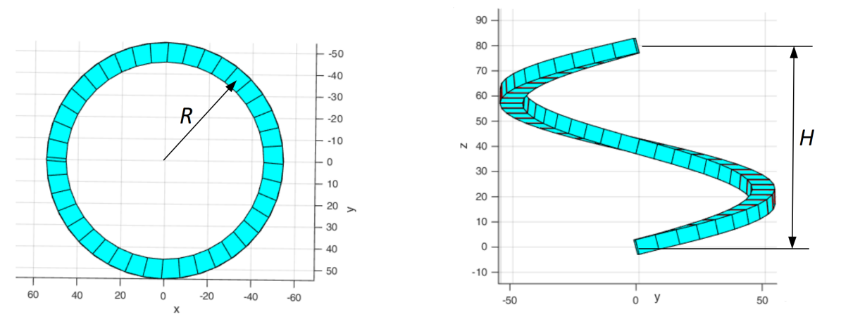
Let us consider again the example from Section 23.1: a clamped curved helicoidal beam is analysed,

R=50\ {\rm mm}, \qquad H=80\ {\rm mm},

with rectangular cross-section

h\times b=9\times6\ {\rm mm}.

Refer to the MATLAB subprogram gen for all input data.

Helicoidal beam geometry — **Figure 2.**

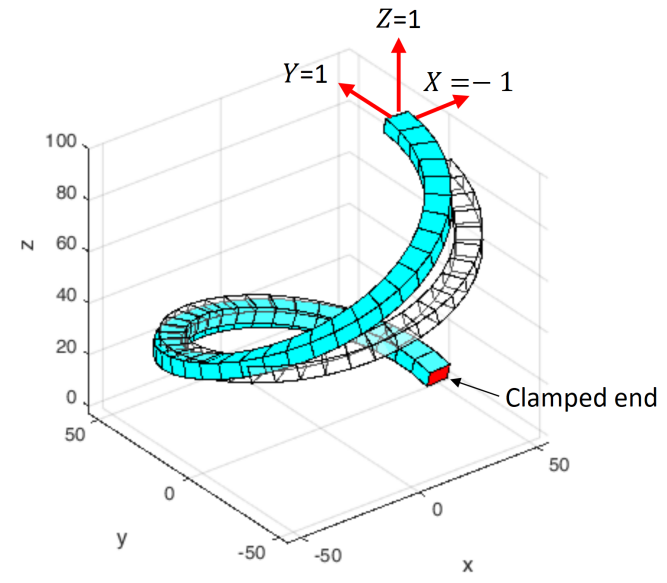
Loaded and deformed helicoidal beam — **Figure 3.**

The displacements of the loaded beam end are:

	Euler–Bernoulli beam model	Timoshenko beam model
$u$	$-9.814$ mm	$-9.824$ mm
$v$	$10.814$ mm	$10.824$ mm
$w$	$17.105$ mm	$17.123$ mm
$\psi_x$	$-0.074273$	$-0.074273$
$\psi_y$	$-0.19325$	$-0.19325$
$\psi_z$	$0.068256$	$0.068256$

Remark. The displacements are given in the global reference frame. The angles $\psi_x,\psi_y,\psi_z$ represent the rotations of the cross-section about the axes of the global reference frame.

As can be seen, the linear displacements are very slightly larger in the case of the Timoshenko beam model, because the shear angles $\beta_y$ and $\beta_z$ are very small, while the rotations are identical.

In both models, the angular degrees of freedom are the rotations of the cross-section. In the Euler–Bernoulli beam model, the rotation of the cross-section coincides with the rotation of the normal.

08 References

1. Andersen, L., Nielsen, S. R. K., Elastic Beams in Three Dimensions, Aalborg University, Department of Civil Engineering, 2008.