Hypotheses:
Strain Small
Displacement Small
Material Linear
Timoshenko beam model.
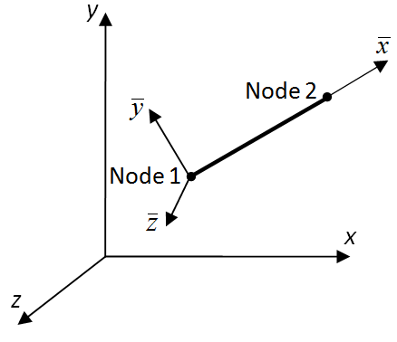
Beam element: straight, prismatic (constant cross-section), two nodes.
The local reference frame contains the beam centroidal axis, the local x ˉ \bar x x ˉ y ˉ \bar y y ˉ z ˉ \bar z z ˉ
In the local reference frame, these DOFs are three displacements
( u ˉ , v ˉ , w ˉ )
(\bar u,\bar v,\bar w)
( u ˉ , v ˉ , w ˉ ) and three rotations of the cross-section
( ψ x ˉ , ψ y ˉ , ψ z ˉ ) .
(\psi_{\bar x},\psi_{\bar y},\psi_{\bar z}).
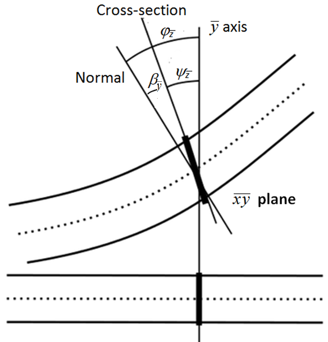
( ψ x ˉ , ψ y ˉ , ψ z ˉ ) . For the Timoshenko beam, the nodal rotations are the rotations of the cross-section ψ x ˉ , ψ y ˉ , ψ z ˉ \psi_{\bar x},\psi_{\bar y},\psi_{\bar z} ψ x ˉ , ψ y ˉ , ψ z ˉ φ x ˉ , φ y ˉ , φ z ˉ \varphi_{\bar x},\varphi_{\bar y},\varphi_{\bar z} φ x ˉ , φ y ˉ , φ z ˉ
Figure 1. The Timoshenko beam is described by the following two groups of equations in the local reference frame.
For the x ˉ y ˉ \bar x\bar y x ˉ y ˉ
{ d ψ z ˉ d x ˉ = M z ˉ E I z , β y = T y G A y , φ z ˉ = d v ˉ d x ˉ , φ z ˉ = ψ z ˉ + β y .
\left\{
\begin{array}{l}
\dfrac{d\psi_{\bar z}}{d\bar x}
=
\dfrac{M_{\bar z}}{EI_z},
\\[3mm]
\beta_y
=
\dfrac{T_y}{GA_y},
\\[3mm]
\varphi_{\bar z}
=
\dfrac{d\bar v}{d\bar x},
\\[3mm]
\varphi_{\bar z}
=
\psi_{\bar z}+\beta_y .
\end{array}
\right.
⎩ ⎨ ⎧ d x ˉ d ψ z ˉ = E I z M z ˉ , β y = G A y T y , φ z ˉ = d x ˉ d v ˉ , φ z ˉ = ψ z ˉ + β y . For the x ˉ z ˉ \bar x\bar z x ˉ z ˉ
{ d ψ y ˉ d x ˉ = M y ˉ E I y , β z = T z ˉ G A z , φ y ˉ = − d w ˉ d x ˉ , φ y ˉ = ψ y ˉ − β z .
\left\{
\begin{array}{l}
\dfrac{d\psi_{\bar y}}{d\bar x}
=
\dfrac{M_{\bar y}}{EI_y},
\\[3mm]
\beta_z
=
\dfrac{T_{\bar z}}{GA_z},
\\[3mm]
\varphi_{\bar y}
=
-\dfrac{d\bar w}{d\bar x},
\\[3mm]
\varphi_{\bar y}
=
\psi_{\bar y}-\beta_z .
\end{array}
\right.
⎩ ⎨ ⎧ d x ˉ d ψ y ˉ = E I y M y ˉ , β z = G A z T z ˉ , φ y ˉ = − d x ˉ d w ˉ , φ y ˉ = ψ y ˉ − β z . β y \beta_y β y β z \beta_z β z φ y ˉ \varphi_{\bar y} φ y ˉ φ z ˉ \varphi_{\bar z} φ z ˉ
01 Isoparametric interpolationThis isoparametric finite element of constant cross-section has two nodes with coordinates:
( x ˉ 1 , y ˉ 1 , z ˉ 1 ) , ( x ˉ 2 , y ˉ 2 , z ˉ 2 ) .
(\bar x_1,\bar y_1,\bar z_1),
\qquad
(\bar x_2,\bar y_2,\bar z_2).
( x ˉ 1 , y ˉ 1 , z ˉ 1 ) , ( x ˉ 2 , y ˉ 2 , z ˉ 2 ) . The coordinates are interpolated along the element using the shape function:
{ x ˉ ( ξ ) y ˉ ( ξ ) z ˉ ( ξ ) } = N ( ξ ) { x ˉ 1 y ˉ 1 z ˉ 1 x ˉ 2 y ˉ 2 z ˉ 2 } .
\left\{
\begin{array}{c}
\bar x(\xi)\\
\bar y(\xi)\\
\bar z(\xi)
\end{array}
\right\}
=
\boldsymbol{N}(\xi)
\left\{
\begin{array}{c}
\bar x_1\\
\bar y_1\\
\bar z_1\\
\bar x_2\\
\bar y_2\\
\bar z_2
\end{array}
\right\}.
⎩ ⎨ ⎧ x ˉ ( ξ ) y ˉ ( ξ ) z ˉ ( ξ ) ⎭ ⎬ ⎫ = N ( ξ ) ⎩ ⎨ ⎧ x ˉ 1 y ˉ 1 z ˉ 1 x ˉ 2 y ˉ 2 z ˉ 2 ⎭ ⎬ ⎫ . The same shape functions are used to interpolate the three displacements and the three rotations of the cross-section along the beam element:
{ u ˉ v ˉ w ˉ ψ x ˉ ψ y ˉ ψ z ˉ } = N ( ξ ) { u ˉ 1 v ˉ 1 w ˉ 1 ψ x ˉ 1 ψ y ˉ 1 ψ z ˉ 1 u ˉ 2 v ˉ 2 w ˉ 2 ψ x ˉ 2 ψ y ˉ 2 ψ z ˉ 2 } .
\left\{
\begin{array}{c}
\bar u\\
\bar v\\
\bar w\\
\psi_{\bar x}\\
\psi_{\bar y}\\
\psi_{\bar z}
\end{array}
\right\}
=
\boldsymbol{N}(\xi)
\left\{
\begin{array}{c}
\bar u_1\\
\bar v_1\\
\bar w_1\\
\psi_{\bar x1}\\
\psi_{\bar y1}\\
\psi_{\bar z1}\\
\bar u_2\\
\bar v_2\\
\bar w_2\\
\psi_{\bar x2}\\
\psi_{\bar y2}\\
\psi_{\bar z2}
\end{array}
\right\}.
⎩ ⎨ ⎧ u ˉ v ˉ w ˉ ψ x ˉ ψ y ˉ ψ z ˉ ⎭ ⎬ ⎫ = N ( ξ ) ⎩ ⎨ ⎧ u ˉ 1 v ˉ 1 w ˉ 1 ψ x ˉ 1 ψ y ˉ 1 ψ z ˉ 1 u ˉ 2 v ˉ 2 w ˉ 2 ψ x ˉ 2 ψ y ˉ 2 ψ z ˉ 2 ⎭ ⎬ ⎫ . The one-dimensional shape functions are linear:
h 1 = 1 − ξ 2 , h 2 = 1 + ξ 2 , ξ ∈ [ − 1 , 1 ] .
h_1=\frac{1-\xi}{2},
\qquad
h_2=\frac{1+\xi}{2},
\qquad
\xi\in[-1,1].
h 1 = 2 1 − ξ , h 2 = 2 1 + ξ , ξ ∈ [ − 1 , 1 ] . Thus,
u ˉ = h 1 u ˉ 1 + h 2 u ˉ 2 ,
\bar u=h_1\bar u_1+h_2\bar u_2,
u ˉ = h 1 u ˉ 1 + h 2 u ˉ 2 , v ˉ = h 1 v ˉ 1 + h 2 v ˉ 2 ,
\bar v=h_1\bar v_1+h_2\bar v_2,
v ˉ = h 1 v ˉ 1 + h 2 v ˉ 2 , w ˉ = h 1 w ˉ 1 + h 2 w ˉ 2 ,
\bar w=h_1\bar w_1+h_2\bar w_2,
w ˉ = h 1 w ˉ 1 + h 2 w ˉ 2 , ψ x ˉ = h 1 ψ x ˉ 1 + h 2 ψ x ˉ 2 ,
\psi_{\bar x}
=
h_1\psi_{\bar x1}
+
h_2\psi_{\bar x2},
ψ x ˉ = h 1 ψ x ˉ 1 + h 2 ψ x ˉ 2 , ψ y ˉ = h 1 ψ y ˉ 1 + h 2 ψ y ˉ 2 ,
\psi_{\bar y}
=
h_1\psi_{\bar y1}
+
h_2\psi_{\bar y2},
ψ y ˉ = h 1 ψ y ˉ 1 + h 2 ψ y ˉ 2 , ψ z ˉ = h 1 ψ z ˉ 1 + h 2 ψ z ˉ 2 .
\psi_{\bar z}
=
h_1\psi_{\bar z1}
+
h_2\psi_{\bar z2}.
ψ z ˉ = h 1 ψ z ˉ 1 + h 2 ψ z ˉ 2 . The angles ψ x ˉ , ψ y ˉ , ψ z ˉ \psi_{\bar x},\psi_{\bar y},\psi_{\bar z} ψ x ˉ , ψ y ˉ , ψ z ˉ
02 Generalized strain vectorThe matrix B \boldsymbol{B} B Section 23.2 :
ε = { ε 0 β y β z κ x ˉ κ y ˉ κ z ˉ } .
\boldsymbol{\varepsilon}
=
\left\{
\begin{array}{c}
\varepsilon_0\\
\beta_y\\
\beta_z\\
\kappa_{\bar x}\\
\kappa_{\bar y}\\
\kappa_{\bar z}
\end{array}
\right\}.
ε = ⎩ ⎨ ⎧ ε 0 β y β z κ x ˉ κ y ˉ κ z ˉ ⎭ ⎬ ⎫ . The generalized strains are
ε 0 = d u ˉ d x ˉ ,
\varepsilon_0
=
\frac{d\bar u}{d\bar x},
ε 0 = d x ˉ d u ˉ , β y = d v ˉ d x ˉ − ψ z ˉ ,
\beta_y
=
\frac{d\bar v}{d\bar x}
-
\psi_{\bar z},
β y = d x ˉ d v ˉ − ψ z ˉ , β z = d w ˉ d x ˉ + ψ y ˉ ,
\beta_z
=
\frac{d\bar w}{d\bar x}
+
\psi_{\bar y},
β z = d x ˉ d w ˉ + ψ y ˉ , κ x ˉ = d ψ x ˉ d x ˉ ,
\kappa_{\bar x}
=
\frac{d\psi_{\bar x}}{d\bar x},
κ x ˉ = d x ˉ d ψ x ˉ , κ y ˉ = d ψ y ˉ d x ˉ ,
\kappa_{\bar y}
=
\frac{d\psi_{\bar y}}{d\bar x},
κ y ˉ = d x ˉ d ψ y ˉ , κ z ˉ = d ψ z ˉ d x ˉ .
\kappa_{\bar z}
=
\frac{d\psi_{\bar z}}{d\bar x}.
κ z ˉ = d x ˉ d ψ z ˉ . Here κ x ˉ , κ y ˉ , κ z ˉ \kappa_{\bar x},\kappa_{\bar y},\kappa_{\bar z} κ x ˉ , κ y ˉ , κ z ˉ
The element nodal displacement vector is
u ‾ e l = { u ˉ 1 v ˉ 1 w ˉ 1 ψ x ˉ 1 ψ y ˉ 1 ψ z ˉ 1 u ˉ 2 v ˉ 2 w ˉ 2 ψ x ˉ 2 ψ y ˉ 2 ψ z ˉ 2 } .
\overline{\boldsymbol{u}}_{el}
=
\left\{
\begin{array}{c}
\bar u_1\\
\bar v_1\\
\bar w_1\\
\psi_{\bar x1}\\
\psi_{\bar y1}\\
\psi_{\bar z1}\\
\bar u_2\\
\bar v_2\\
\bar w_2\\
\psi_{\bar x2}\\
\psi_{\bar y2}\\
\psi_{\bar z2}
\end{array}
\right\}.
u e l = ⎩ ⎨ ⎧ u ˉ 1 v ˉ 1 w ˉ 1 ψ x ˉ 1 ψ y ˉ 1 ψ z ˉ 1 u ˉ 2 v ˉ 2 w ˉ 2 ψ x ˉ 2 ψ y ˉ 2 ψ z ˉ 2 ⎭ ⎬ ⎫ . Hence,
ε = B u ‾ e l .
\boxed{
\boldsymbol{\varepsilon}
=
\boldsymbol{B}\,
\overline{\boldsymbol{u}}_{el}
}.
ε = B u e l . 03 Derivatives of the shape functionsThe beam-element length is
L = x ˉ 2 − x ˉ 1 .
L=\bar x_2-\bar x_1.
L = x ˉ 2 − x ˉ 1 . Since
d ξ d x ˉ = 2 L ,
\frac{d\xi}{d\bar x}
=
\frac{2}{L},
d x ˉ d ξ = L 2 , we obtain
d h 1 d x ˉ = − 1 L , d h 2 d x ˉ = 1 L .
\frac{dh_1}{d\bar x}
=
-\frac{1}{L},
\qquad
\frac{dh_2}{d\bar x}
=
\frac{1}{L}.
d x ˉ d h 1 = − L 1 , d x ˉ d h 2 = L 1 . Consequently,
ε 0 = u ˉ 2 − u ˉ 1 L ,
\varepsilon_0
=
\frac{\bar u_2-\bar u_1}{L},
ε 0 = L u ˉ 2 − u ˉ 1 , β y = − v ˉ 1 L − h 1 ψ z ˉ 1 + v ˉ 2 L − h 2 ψ z ˉ 2 ,
\beta_y
=
-\frac{\bar v_1}{L}
-h_1\psi_{\bar z1}
+
\frac{\bar v_2}{L}
-h_2\psi_{\bar z2},
β y = − L v ˉ 1 − h 1 ψ z ˉ 1 + L v ˉ 2 − h 2 ψ z ˉ 2 , β z = − w ˉ 1 L + h 1 ψ y ˉ 1 + w ˉ 2 L + h 2 ψ y ˉ 2 ,
\beta_z
=
-\frac{\bar w_1}{L}
+h_1\psi_{\bar y1}
+
\frac{\bar w_2}{L}
+h_2\psi_{\bar y2},
β z = − L w ˉ 1 + h 1 ψ y ˉ 1 + L w ˉ 2 + h 2 ψ y ˉ 2 , κ x ˉ = − ψ x ˉ 1 L + ψ x ˉ 2 L ,
\kappa_{\bar x}
=
-\frac{\psi_{\bar x1}}{L}
+
\frac{\psi_{\bar x2}}{L},
κ x ˉ = − L ψ x ˉ 1 + L ψ x ˉ 2 , κ y ˉ = − ψ y ˉ 1 L + ψ y ˉ 2 L ,
\kappa_{\bar y}
=
-\frac{\psi_{\bar y1}}{L}
+
\frac{\psi_{\bar y2}}{L},
κ y ˉ = − L ψ y ˉ 1 + L ψ y ˉ 2 , κ z ˉ = − ψ z ˉ 1 L + ψ z ˉ 2 L .
\kappa_{\bar z}
=
-\frac{\psi_{\bar z1}}{L}
+
\frac{\psi_{\bar z2}}{L}.
κ z ˉ = − L ψ z ˉ 1 + L ψ z ˉ 2 . Finally,
B ( ξ ) = [ − 1 L 0 0 0 0 0 1 L 0 0 0 0 0 0 − 1 L 0 0 0 − h 1 0 1 L 0 0 0 − h 2 0 0 − 1 L 0 h 1 0 0 0 1 L 0 h 2 0 0 0 0 − 1 L 0 0 0 0 0 1 L 0 0 0 0 0 0 − 1 L 0 0 0 0 0 1 L 0 0 0 0 0 0 − 1 L 0 0 0 0 0 1 L ] .
\boxed{
\boldsymbol{B}(\xi)=
\begin{bmatrix}
-\dfrac1L&0&0&0&0&0&
\dfrac1L&0&0&0&0&0
\\[3mm]
0&-\dfrac1L&0&0&0&-h_1&
0&\dfrac1L&0&0&0&-h_2
\\[3mm]
0&0&-\dfrac1L&0&h_1&0&
0&0&\dfrac1L&0&h_2&0
\\[3mm]
0&0&0&-\dfrac1L&0&0&
0&0&0&\dfrac1L&0&0
\\[3mm]
0&0&0&0&-\dfrac1L&0&
0&0&0&0&\dfrac1L&0
\\[3mm]
0&0&0&0&0&-\dfrac1L&
0&0&0&0&0&\dfrac1L
\end{bmatrix}.
}
B ( ξ ) = − L 1 0 0 0 0 0 0 − L 1 0 0 0 0 0 0 − L 1 0 0 0 0 0 0 − L 1 0 0 0 0 h 1 0 − L 1 0 0 − h 1 0 0 0 − L 1 L 1 0 0 0 0 0 0 L 1 0 0 0 0 0 0 L 1 0 0 0 0 0 0 L 1 0 0 0 0 h 2 0 L 1 0 0 − h 2 0 0 0 L 1 . 04 Hooke’s lawHooke’s law in matrix form is
σ = D ε ,
\boldsymbol{\sigma}
=
\boldsymbol{D}
\boldsymbol{\varepsilon},
σ = D ε , where
σ = { N T y T z M x ˉ M y ˉ M z ˉ } ,
\boldsymbol{\sigma}
=
\left\{
\begin{array}{c}
N\\
T_y\\
T_z\\
M_{\bar x}\\
M_{\bar y}\\
M_{\bar z}
\end{array}
\right\},
σ = ⎩ ⎨ ⎧ N T y T z M x ˉ M y ˉ M z ˉ ⎭ ⎬ ⎫ , and
D = [ E A 0 0 0 0 0 0 G A y 0 0 0 0 0 0 G A z 0 0 0 0 0 0 G I t 0 0 0 0 0 0 E I y 0 0 0 0 0 0 E I z ] .
\boldsymbol{D}=
\begin{bmatrix}
EA&0&0&0&0&0\\
0&GA_y&0&0&0&0\\
0&0&GA_z&0&0&0\\
0&0&0&GI_t&0&0\\
0&0&0&0&EI_y&0\\
0&0&0&0&0&EI_z
\end{bmatrix}.
D = E A 0 0 0 0 0 0 G A y 0 0 0 0 0 0 G A z 0 0 0 0 0 0 G I t 0 0 0 0 0 0 E I y 0 0 0 0 0 0 E I z . 05 Element stiffness matrixThe stiffness matrix in the local reference frame is
k ‾ e l = ∫ L B T D B d x ˉ .
\boxed{
\overline{\boldsymbol{k}}_{el}
=
\int_L
\boldsymbol{B}^T
\boldsymbol{D}
\boldsymbol{B}\,
d\bar x
}.
k e l = ∫ L B T D B d x ˉ . Because B \boldsymbol{B} B ξ \xi ξ
For
the element stiffness matrix is evaluated as
k ‾ e l = L B ( 0 ) T D B ( 0 ) .
\boxed{
\overline{\boldsymbol{k}}_{el}
=
L\,
\boldsymbol{B}(0)^T
\boldsymbol{D}
\boldsymbol{B}(0)
}.
k e l = L B ( 0 ) T D B ( 0 ) . 06 Shear-stiffness modificationTo improve the accuracy of this two-node isoparametric beam element, we introduce the same correction used in Section 5.3 .
The shear stiffnesses are modified as follows:
G A y ⟶ γ y G A y ,
GA_y
\longrightarrow
\gamma_y GA_y,
G A y ⟶ γ y G A y , G A z ⟶ γ z G A z ,
GA_z
\longrightarrow
\gamma_z GA_z,
G A z ⟶ γ z G A z , where
γ y = Φ y 1 + Φ y
\boxed{
\gamma_y=\frac{\Phi_y}{1+\Phi_y}
}
γ y = 1 + Φ y Φ y and
Φ y = 12 E I z G A y L 2 ,
\boxed{
\Phi_y=
\frac{12EI_z}{GA_yL^2}
},
Φ y = G A y L 2 12 E I z , while
γ z = Φ z 1 + Φ z
\boxed{
\gamma_z=\frac{\Phi_z}{1+\Phi_z}
}
γ z = 1 + Φ z Φ z and
Φ z = 12 E I y G A z L 2 .
\boxed{
\Phi_z=
\frac{12EI_y}{GA_zL^2}
}.
Φ z = G A z L 2 12 E I y . With this modification, the two-node isoparametric Timoshenko beam gives the same results as the finite element presented in Section 23.2 .
07 Transformation to the global reference frameThe same passive rotation convention as in Section 23.1 is used:
u ‾ e l = R u e l ,
\overline{\boldsymbol{u}}_{el}
=
\boldsymbol{R}
\boldsymbol{u}_{el},
u e l = R u e l , where R \boldsymbol{R} R
Consequently,
k e l = R T k ‾ e l R .
\boxed{
\boldsymbol{k}_{el}
=
\boldsymbol{R}^T
\overline{\boldsymbol{k}}_{el}
\boldsymbol{R}
}.
k e l = R T k e l R . Refer to Section 23.1 for details regarding the construction of R \boldsymbol{R} R
The results obtained using the finite element presented in this section are identical to those obtained with the finite element described in Section 23.2 .
A MATLAB computer code is available for download.
MATLAB Two-node isoparametric beam element — Timoshenko model Download ZIP PREVIOUS SECTION ← 23.2. 3D beam element. Timoshenko model NEXT SECTION 23.4. Differential equilibrium equations for 3D slender curved beams →