5.1 Beam Finite Element — Euler–Bernoulli Beam Model

Model and notation

The element is straight and prismatic, with two nodes and a constant cross-section. Each node has two translations and one rotation. The analysis is performed in the global $xy$ plane.

In this planar analysis, $T$ and $T_y$ denote the same transverse force component, while $M$ and $M_z$ denote the same bending moment component.

01Small strains

02Small displacements

03Linear elastic material

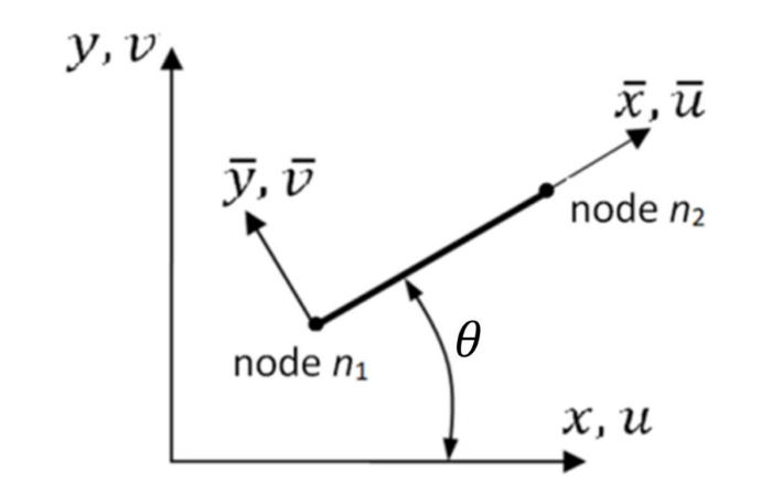
The local $\bar{x}$ axis coincides with the neutral axis. The local $\bar{y}$ axis is a principal axis of the cross-section, and $\theta$ is the angle from the global frame to the local frame.

Two-node beam element with global and local coordinate systems and displacement components — Figure 1. Global and local coordinate systems and positive element displacement components.

The local and global element displacement vectors are:

\bar{\boldsymbol{u}}_{el}=\left\{\begin{array}{c}\bar{u}_1\\\bar{v}_1\\\varphi_1\\\bar{u}_2\\\bar{v}_2\\\varphi_2\end{array}\right\}

\boldsymbol{u}_{el}=\left\{\begin{array}{c}u_1\\v_1\\\varphi_1\\u_2\\v_2\\\varphi_2\end{array}\right\}

In accordance with the site-wide beam convention, the axial strain of the neutral axis, the rotation, and the curvature are:

\varepsilon_0=\frac{d\bar{u}}{d\bar{x}},\qquad \varphi_z=\frac{d\bar{v}}{d\bar{x}},\qquad \kappa_z=\frac{d\varphi_z}{d\bar{x}}=\frac{d^2\bar{v}}{d\bar{x}^2}

Thus positive curvature is consistent with the convention inNomenclature and Conventions. The generalized constitutive relation is:

\boldsymbol{\sigma}=\boldsymbol{D}\boldsymbol{\varepsilon},\qquad \left\{\begin{array}{c}N\\M_z\end{array}\right\}=\left[\begin{array}{cc}EA&0\\0&EI_z\end{array}\right]\left\{\begin{array}{c}\varepsilon_0\\\kappa_z\end{array}\right\}

Here N is the axial force, M_z is the bending moment, E is Young's modulus, and A andI_z are the cross-sectional area and second moment of area.

Classical approach

Let $\xi=\bar{x}/L$ , with $0\leq\xi\leq1$ . Linear interpolation is used for the axial displacement, while cubic Hermite interpolation is used for the transverse displacement. The rotation follows by differentiation[1] [2].

\left\{\begin{array}{c}\bar{u}(\bar{x})\\\bar{v}(\bar{x})\\\varphi_z(\bar{x})\end{array}\right\}=\boldsymbol{N}(\xi)\bar{\boldsymbol{u}}_{el}

\boldsymbol{N}(\xi)=\left[\begin{array}{cccccc}1-\xi&0&0&\xi&0&0\\0&2\xi^3-3\xi^2+1&(\xi^3-2\xi^2+\xi)L&0&-2\xi^3+3\xi^2&(\xi^3-\xi^2)L\\0&(6\xi^2-6\xi)/L&3\xi^2-4\xi+1&0&(-6\xi^2+6\xi)/L&3\xi^2-2\xi\end{array}\right]

The generalized strain vector is:

\boldsymbol{\varepsilon}(\bar{x})=\left\{\begin{array}{c}\varepsilon_0\\\kappa_z\end{array}\right\}=\boldsymbol{B}(\xi)\bar{\boldsymbol{u}}_{el}

\boldsymbol{B}(\xi)=\left[\begin{array}{cccccc}-1/L&0&0&1/L&0&0\\0&(12\xi-6)/L^2&(6\xi-4)/L&0&(-12\xi+6)/L^2&(6\xi-2)/L\end{array}\right]

Deformation energy and stiffness matrix

The deformation energy of one element is:

U_{el}=\frac{1}{2}\int_0^L\boldsymbol{\varepsilon}^{T}\boldsymbol{D}\boldsymbol{\varepsilon}\,d\bar{x}=\frac{1}{2}\bar{\boldsymbol{u}}_{el}^{T}\bar{\boldsymbol{k}}_{el}\bar{\boldsymbol{u}}_{el}

\bar{\boldsymbol{k}}_{el}=\frac{\partial^2U_{el}}{\partial\bar{\boldsymbol{u}}_{el}^{2}}=\int_0^L\boldsymbol{B}^{T}\boldsymbol{D}\boldsymbol{B}\,d\bar{x}

After exact integration,

\bar{\boldsymbol{k}}_{el}=\left[\begin{array}{cccccc}EA/L&0&0&-EA/L&0&0\\0&12EI_z/L^3&6EI_z/L^2&0&-12EI_z/L^3&6EI_z/L^2\\0&6EI_z/L^2&4EI_z/L&0&-6EI_z/L^2&2EI_z/L\\-EA/L&0&0&EA/L&0&0\\0&-12EI_z/L^3&-6EI_z/L^2&0&12EI_z/L^3&-6EI_z/L^2\\0&6EI_z/L^2&2EI_z/L&0&-6EI_z/L^2&4EI_z/L\end{array}\right]

The transformation from global to local element coordinates is:

\bar{\boldsymbol{u}}_{el}=\boldsymbol{R}\boldsymbol{u}_{el},\qquad \boldsymbol{R}=\left[\begin{array}{cc}\boldsymbol{R}_0&\boldsymbol{0}_{3\times3}\\\boldsymbol{0}_{3\times3}&\boldsymbol{R}_0\end{array}\right]

\boldsymbol{R}_0=\left[\begin{array}{ccc}\cos\theta&\sin\theta&0\\-\sin\theta&\cos\theta&0\\0&0&1\end{array}\right]

The stiffness matrix in the global frame is:

\boldsymbol{k}_{el}=\boldsymbol{R}^{T}\bar{\boldsymbol{k}}_{el}\boldsymbol{R}

Energy formulation with Gaussian quadrature

The same stiffness matrix can be obtained by differentiating the deformation energy directly. This form is particularly convenient when the formulation is later extended to nonlinear problems.

U_{el}=\frac{1}{2}\int_0^L\left(EA\varepsilon_0^2+EI_z\kappa_z^2\right)\,d\bar{x}

U_{el}=\frac{L}{4}\sum_{G=1}^{n_G}w_G\left[EA\varepsilon_0(\xi_G)^2+EI_z\kappa_z(\xi_G)^2\right]

Two Gauss points give the exact result because the highest-order term in the integrand is quadratic. On $0\leq\xi\leq1$ , their coordinates and weights are:

\xi_{1,2}=\frac{1}{2}\left(1\mp\frac{1}{\sqrt{3}}\right),\qquad w_1=w_2=1

\bar{\boldsymbol{k}}_{el}=\frac{L}{2}\sum_{G=1}^{2}\left[EA\frac{\partial\varepsilon_0}{\partial\bar{\boldsymbol{u}}_{el}}\left(\frac{\partial\varepsilon_0}{\partial\bar{\boldsymbol{u}}_{el}}\right)^{T}+EI_z\frac{\partial\kappa_z}{\partial\bar{\boldsymbol{u}}_{el}}\left(\frac{\partial\kappa_z}{\partial\bar{\boldsymbol{u}}_{el}}\right)^{T}\right]

The derivative vectors evaluated at each Gauss point are:

\frac{\partial\varepsilon_0}{\partial\bar{\boldsymbol{u}}_{el}}=\left\{\begin{array}{c}-1/L\\0\\0\\1/L\\0\\0\end{array}\right\}

\frac{\partial\kappa_z}{\partial\bar{\boldsymbol{u}}_{el}}=\left\{\begin{array}{c}0\\(12\xi-6)/L^2\\(6\xi-4)/L\\0\\(-12\xi+6)/L^2\\(6\xi-2)/L\end{array}\right\}

Numerical example

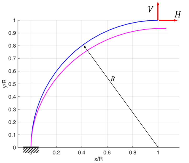
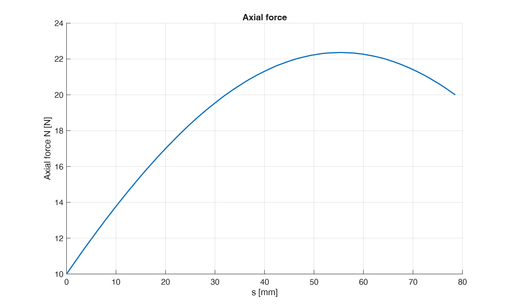
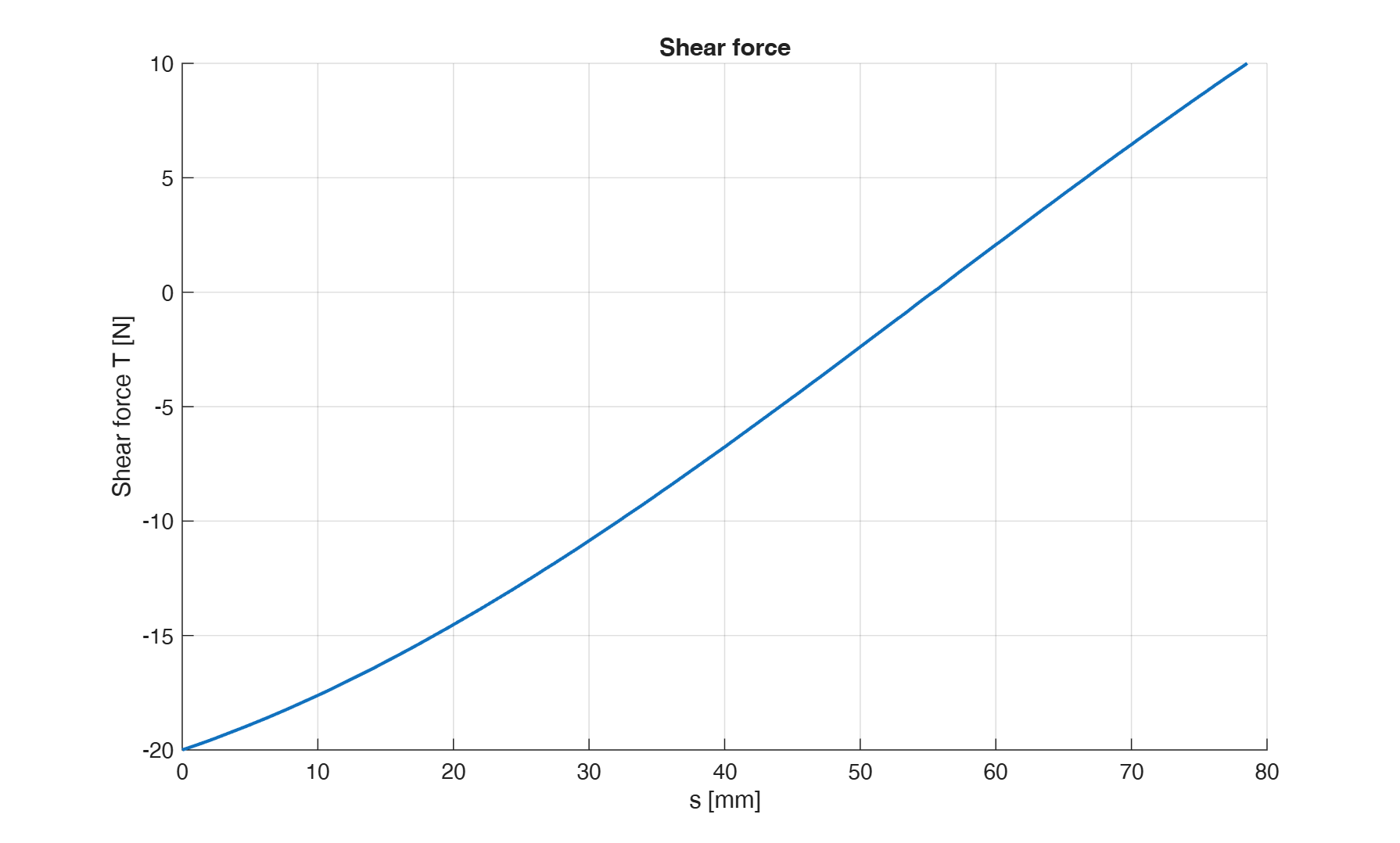
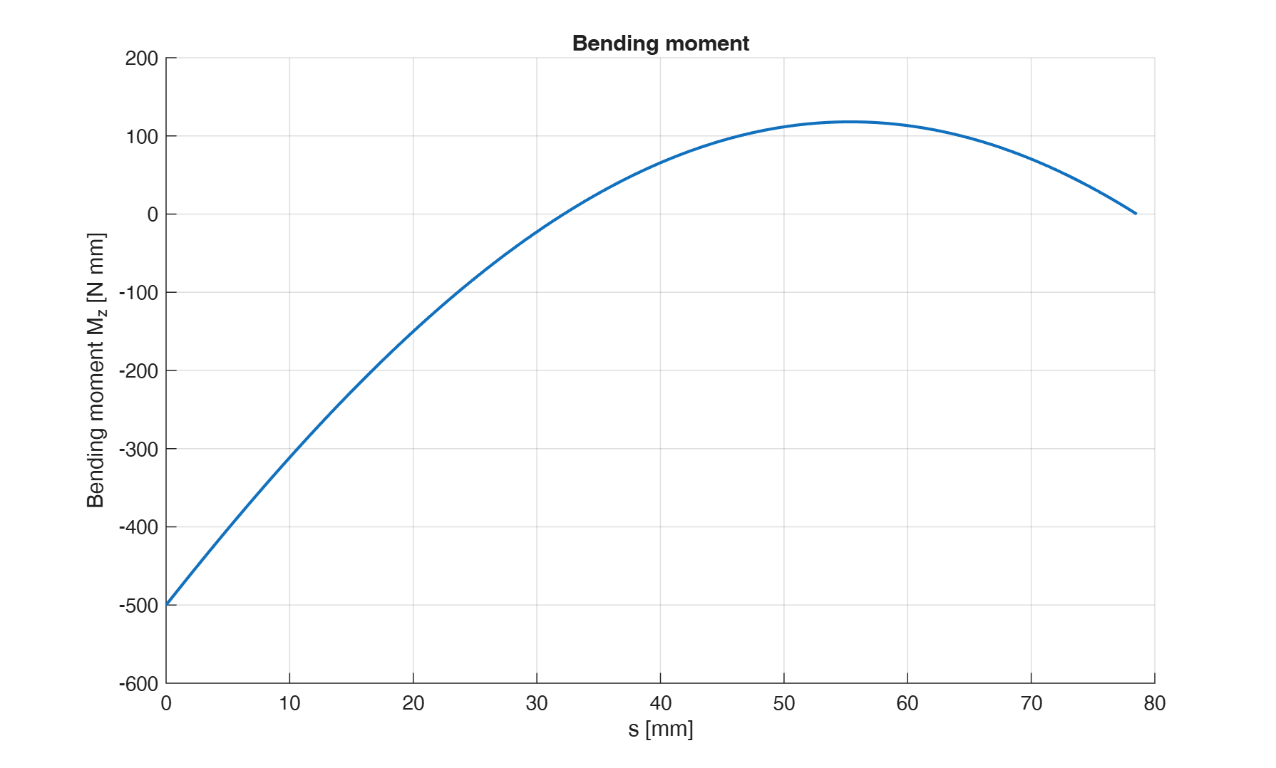
A quarter-circular cantilever of radius $R=50\ \mathrm{mm}$ is discretized with 100 straight beam elements. The rectangular cross-section has width $w=5\ \mathrm{mm}$ and thickness $t=1\ \mathrm{mm}$ . The material and tip loads are $E=2\times10^5\ \mathrm{MPa}$ , $V=10\ \mathrm{N}$ , and $H=20\ \mathrm{N}$ .

Undeformed and deformed quarter-circular cantilever under horizontal and vertical tip forces — Figure 2. Undeformed and deformed beam centreline. The displacements are shown at their true scale.

Axial-force diagram — Figure 3. Axial force N.

Shear-force diagram — Figure 4. Shear force T_y.

Bending-moment diagram — Figure 5. Bending moment M_z.

MATLAB programs

The package contains five commented files. gen.mdefines the geometry, cross-section, loads, and constraints;deriv.m evaluates the axial-strain and curvature-displacement matrices; stiff.m performs two-point Gauss integration and global assembly;stress.m recovers the internal force resultants; and main.m controls the analysis and plots the results.

The implementation uses the same positive-curvature convention as the derivation above. Accordingly, deriv.mevaluates κ_z = d²v/dx², whilestress.m recovers the shear force from dM_z/dx = −T_y.

stiff.mTwo-point Gauss integration

% Local stiffness matrix in the current element frame.
for ig = 1:2
    xc = 1/2*(1 + xg(ig));
    deriv
    kel = kel + L/2*(ea*ep1*ep1' + ei*ka1*ka1');
end
K(ip,ip) = K(ip,ip) + Re'*kel*Re;

MATLAB compatibility

Tested in MATLAB R2024a. The code uses standard MATLAB syntax and is expected to be compatible with newer MATLAB versions. No additional toolbox is required.

MEuler–Bernoulli beam MATLAB package5 commented MATLAB files and README · tested in R2024aDownload ZIP

References

O. C. Zienkiewicz, R. L. Taylor, and J. Z. Zhu, The Finite Element Method: Its Basis and Fundamentals, 7th ed., Elsevier, 2013.
K. J. Bathe, Finite Element Procedures, 2nd ed., Klaus-Jürgen Bathe, 2014.