Section 5.2 of Chapter 5: 2D Beam Element, Linear Case

Beam Finite Element — Timoshenko Beam Model

A two-node planar beam element with axial deformation, bending deformation, and transverse shear deformation.

2D beamTimoshenkoLinear analysisMATLAB

01

Model and kinematics

A straight, prismatic two-node beam element of constant cross-section is analysed in the global xyxy plane. Small strains, small displacements, and linear elastic material behaviour are assumed [1].

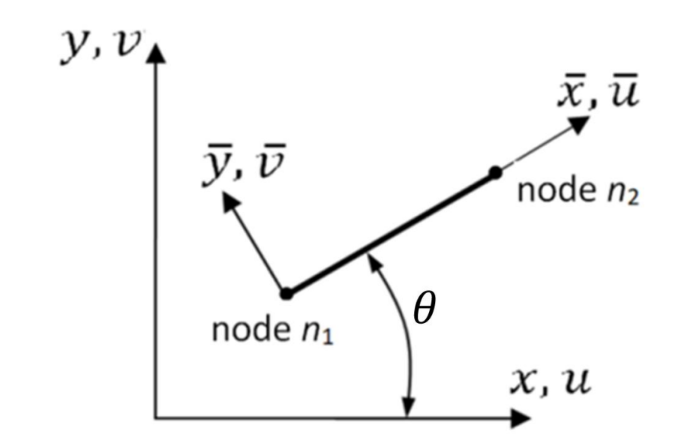
The local xˉ\bar x axis coincides with the neutral axis of the element, while yˉ\bar y is a principal axis of the cross-section. The angle θ\theta defines the orientation of the local frame with respect to the global frame.

Two-node beam element with global and local coordinate systems and displacement components
Figure 1. Global and local coordinate systems and positive element displacement components.
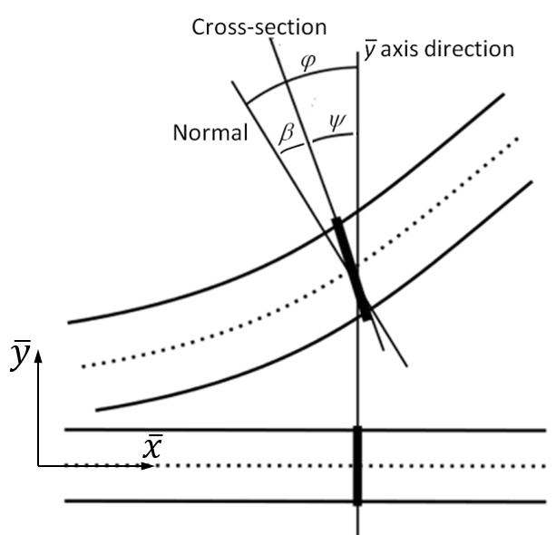
Timoshenko beam cross-section showing the normal, the cross-section, and their rotations
Figure 2. Timoshenko kinematic quantities at a cross-section: normal rotation φ, cross-section rotation ψ, and shear angle β.

Each node has the local degrees of freedom uˉ\bar u, vˉ\bar v, and ψ\psi. The global nodal displacement components are uu, vv, and ψ\psi. The local element vector is:

uˉel={uˉ1vˉ1ψ1uˉ2vˉ2ψ2}\bar{\boldsymbol u}_{el}=\begin{Bmatrix}\bar u_1\\[3pt]\bar v_1\\[3pt]\psi_1\\[3pt]\bar u_2\\[3pt]\bar v_2\\[3pt]\psi_2\end{Bmatrix}

The rotation angle of the normal, the rotation angle of the cross-section, and the shear angle have the following expressions:

φ=dvˉdxˉ,ψ=φβ,β=TGA0\varphi=\frac{d\bar v}{d\bar x},\qquad \psi=\varphi-\beta,\qquad \beta=\frac{T}{GA_0}

The rotation of the cross-section is related to the bending moment by:

dψdxˉ=MEI\frac{d\psi}{d\bar x}=\frac{M}{EI}

The nodal angular degree of freedom is ψ\psi, the rotation of the cross-section, not φ\varphi, the rotation of the normal.

The Euler–Bernoulli model is recovered when β=0\beta=0, so that φ=ψ\varphi=\psi.

02

Generalized strains and stresses

For the Timoshenko beam, the generalized strain vector and its work-conjugate generalized stress vector are:

ε={ε0,β,κ}T,σ={N,T,M}T,σ=Dε\boldsymbol{\varepsilon}=\left\{\varepsilon_0,\beta,\kappa\right\}^{T},\qquad \boldsymbol{\sigma}=\left\{N,T,M\right\}^{T},\qquad \boldsymbol{\sigma}=\boldsymbol D\boldsymbol{\varepsilon}
ε0=duˉdxˉ,β=dvˉdxˉψ,κ=dψdxˉ,D=[EA000GA0000EI]\varepsilon_0=\frac{d\bar u}{d\bar x},\qquad \beta=\frac{d\bar v}{d\bar x}-\psi,\qquad \kappa=\frac{d\psi}{d\bar x},\qquad \boldsymbol D=\left[\begin{array}{ccc}EA&0&0\\[4pt]0&GA_0&0\\[4pt]0&0&EI\end{array}\right]
{NTM}=[EA000GA0000EI]{ε0βκ}\left\{\begin{array}{c}N\\[4pt]T\\[4pt]M\end{array}\right\}=\left[\begin{array}{ccc}EA&0&0\\[4pt]0&GA_0&0\\[4pt]0&0&EI\end{array}\right]\left\{\begin{array}{c}\varepsilon_0\\[4pt]\beta\\[4pt]\kappa\end{array}\right\}

Here E and G are Young's modulus and the shear modulus; A, A0A_0, and I are the cross-sectional area, effective shear area, and second moment of area. The generalized strains are the axial strain ε0\varepsilon_0, shear angle β\beta, and curvature κ\kappa. Their work-conjugate generalized stresses are the axial force N, shear force T, and bending moment M.

For the nodal-load case used below, the shear force and therefore β\beta are constant within an element. Consequently,

dβdxˉ=0,dψdxˉ=dφdxˉ,M=EIdφdxˉ\frac{d\beta}{d\bar x}=0,\qquad \frac{d\psi}{d\bar x}=\frac{d\varphi}{d\bar x},\qquad M=EI\frac{d\varphi}{d\bar x}
T=dMdxˉ=EId2φdxˉ2=EId3vˉdxˉ3T=-\frac{dM}{d\bar x}=-EI\frac{d^2\varphi}{d\bar x^2}=-EI\frac{d^3\bar v}{d\bar x^3}

Combining the shear constitutive relation with equilibrium gives:

β=TGA0=EIGA0d3vˉdxˉ3\beta=\frac{T}{GA_0}=-\frac{EI}{GA_0}\frac{d^3\bar v}{d\bar x^3}

03

Interpolation

Let ξ=xˉ/L\xi=\bar x/L, with 0ξ10\leq\xi\leq1. Linear interpolation is used for the axial displacement and cubic interpolation for the transverse displacement:

vˉ(ξ)=[0, 2ξ33ξ2+1, (ξ32ξ2+ξ)L, 0, 2ξ3+3ξ2, (ξ3ξ2)L]{uˉ1,vˉ1,ψ1+β,uˉ2,vˉ2,ψ2+β}T\bar v(\xi)=\left[0,\ 2\xi^3-3\xi^2+1,\ (\xi^3-2\xi^2+\xi)L,\ 0,\ -2\xi^3+3\xi^2,\ (\xi^3-\xi^2)L\right]\left\{\bar u_1,\bar v_1,\psi_1+\beta,\bar u_2,\bar v_2,\psi_2+\beta\right\}^{T}

The interpolation uses the normal rotations φ1=ψ1+β\varphi_1=\psi_1+\beta and φ2=ψ2+β\varphi_2=\psi_2+\beta. Applying the third derivative to the cubic polynomial and using the shear relation gives:

β=EIGA0[0, 12L3, 6L2, 0, 12L3, 6L2]{uˉ1vˉ1ψ1+βuˉ2vˉ2ψ2+β}\beta=\frac{EI}{GA_0}\left[0,\ -\frac{12}{L^3},\ -\frac{6}{L^2},\ 0,\ \frac{12}{L^3},\ -\frac{6}{L^2}\right]\left\{\begin{array}{c}\bar u_1\\\bar v_1\\\psi_1+\beta\\\bar u_2\\\bar v_2\\\psi_2+\beta\end{array}\right\}

Because β\beta occurs on both sides, the preceding equation is solved for β\beta. The result is:

β=Bβuˉel\beta=\boldsymbol B_{\beta}\bar{\boldsymbol u}_{el}
Bε=[1/L, 0, 0, 1/L, 0, 0]\boldsymbol B_{\varepsilon}=\left[-1/L,\ 0,\ 0,\ 1/L,\ 0,\ 0\right]
Bβ=1GA0L2+12EI[0, 12EI/L, 6EI, 0, 12EI/L, 6EI]\boldsymbol B_{\beta}=\frac{1}{GA_0L^2+12EI}\left[0,\ -12EI/L,\ -6EI,\ 0,\ 12EI/L,\ -6EI\right]

The curvature is first obtained by differentiating the normal rotation:

κ=dψdxˉ=dφdxˉ=d2vˉdxˉ2\kappa=\frac{d\psi}{d\bar x}=\frac{d\varphi}{d\bar x}=\frac{d^2\bar v}{d\bar x^2}
κ=[0, 12ξ6L2, 6ξ4L, 0, 12ξ+6L2, 6ξ2L]{uˉ1vˉ1ψ1+βuˉ2vˉ2ψ2+β}\kappa=\left[0,\ \frac{12\xi-6}{L^2},\ \frac{6\xi-4}{L},\ 0,\ \frac{-12\xi+6}{L^2},\ \frac{6\xi-2}{L}\right]\left\{\begin{array}{c}\bar u_1\\\bar v_1\\\psi_1+\beta\\\bar u_2\\\bar v_2\\\psi_2+\beta\end{array}\right\}

Substitution of β=Bβuˉel\beta=\boldsymbol B_{\beta}\bar{\boldsymbol u}_{el} eliminates the additional quantity and yields:

κ=Bκuˉel\kappa=\boldsymbol B_{\kappa}\bar{\boldsymbol u}_{el}
Bκ=1GA0L2+12EI[0, 6GA0(2ξ1), (4GA06GA0ξ)L2+12EIL, 0, 6GA0(2ξ1), (6GA0ξ2GA0)L2+12EIL]\boldsymbol B_{\kappa}=\frac{1}{GA_0L^2+12EI}\left[0,\ 6GA_0(2\xi-1),\ -\frac{(4GA_0-6GA_0\xi)L^2+12EI}{L},\ 0,\ -6GA_0(2\xi-1),\ \frac{(6GA_0\xi-2GA_0)L^2+12EI}{L}\right]

The generalized strains are therefore collected without further approximation:

ε(ξ)={ε0βκ}=B(ξ)uˉel,B=[BεBβBκ]\boldsymbol{\varepsilon}(\xi)=\left\{\begin{array}{c}\varepsilon_0\\\beta\\\kappa\end{array}\right\}=\boldsymbol B(\xi)\bar{\boldsymbol u}_{el},\qquad \boldsymbol B=\left[\begin{array}{c}\boldsymbol B_{\varepsilon}\\\boldsymbol B_{\beta}\\\boldsymbol B_{\kappa}\end{array}\right]
B=[1/L001/L00012EIGA0L3+12EIL6EIGA0L2+12EI012EIGA0L3+12EIL6EIGA0L2+12EI06GA0(2ξ1)GA0L2+12EIGA0(46ξ)L2+12EIGA0L3+12EIL06GA0(2ξ1)GA0L2+12EIGA0(6ξ2)L2+12EIGA0L3+12EIL]\boldsymbol B=\left[\begin{array}{cccccc}-1/L&0&0&1/L&0&0\\[7pt]0&-\dfrac{12EI}{GA_0L^3+12EIL}&-\dfrac{6EI}{GA_0L^2+12EI}&0&\dfrac{12EI}{GA_0L^3+12EIL}&-\dfrac{6EI}{GA_0L^2+12EI}\\[7pt]0&\dfrac{6GA_0(2\xi-1)}{GA_0L^2+12EI}&-\dfrac{GA_0(4-6\xi)L^2+12EI}{GA_0L^3+12EIL}&0&-\dfrac{6GA_0(2\xi-1)}{GA_0L^2+12EI}&\dfrac{GA_0(6\xi-2)L^2+12EI}{GA_0L^3+12EIL}\end{array}\right]

04

Stiffness matrix

The local stiffness follows from the deformation energy:

Uel=120LεTDεdxˉ,kˉel=0LBTDBdxˉU_{el}=\frac{1}{2}\int_0^L\boldsymbol{\varepsilon}^{T}\boldsymbol D\boldsymbol{\varepsilon}\,d\bar x,\qquad \bar{\boldsymbol k}_{el}=\int_0^L\boldsymbol B^{T}\boldsymbol D\boldsymbol B\,d\bar x

Direct integration gives the complete local matrix [2]

kˉel=[EAL00EAL00012EIL3(1+λ)6EIL2(1+λ)012EIL3(1+λ)6EIL2(1+λ)06EIL2(1+λ)(4+λ)EIL(1+λ)06EIL2(1+λ)(2λ)EIL(1+λ)EAL00EAL00012EIL3(1+λ)6EIL2(1+λ)012EIL3(1+λ)6EIL2(1+λ)06EIL2(1+λ)(2λ)EIL(1+λ)06EIL2(1+λ)(4+λ)EIL(1+λ)],λ=12EIGA0L2\bar{\boldsymbol k}_{el}=\left[\begin{array}{cccccc}\dfrac{EA}{L}&0&0&-\dfrac{EA}{L}&0&0\\[7pt]0&\dfrac{12EI}{L^3(1+\lambda)}&\dfrac{6EI}{L^2(1+\lambda)}&0&-\dfrac{12EI}{L^3(1+\lambda)}&\dfrac{6EI}{L^2(1+\lambda)}\\[7pt]0&\dfrac{6EI}{L^2(1+\lambda)}&\dfrac{(4+\lambda)EI}{L(1+\lambda)}&0&-\dfrac{6EI}{L^2(1+\lambda)}&\dfrac{(2-\lambda)EI}{L(1+\lambda)}\\[7pt]-\dfrac{EA}{L}&0&0&\dfrac{EA}{L}&0&0\\[7pt]0&-\dfrac{12EI}{L^3(1+\lambda)}&-\dfrac{6EI}{L^2(1+\lambda)}&0&\dfrac{12EI}{L^3(1+\lambda)}&-\dfrac{6EI}{L^2(1+\lambda)}\\[7pt]0&\dfrac{6EI}{L^2(1+\lambda)}&\dfrac{(2-\lambda)EI}{L(1+\lambda)}&0&-\dfrac{6EI}{L^2(1+\lambda)}&\dfrac{(4+\lambda)EI}{L(1+\lambda)}\end{array}\right],\qquad \lambda=\frac{12EI}{GA_0L^2}

With λ=12EI/(GA0L2)\lambda=12EI/(GA_0L^2), the bending-and-shear terms can be written compactly as:

a=12EIL3(1+λ),b=6EIL2(1+λ),c=(4+λ)EIL(1+λ),d=(2λ)EIL(1+λ)a=\frac{12EI}{L^3(1+\lambda)},\qquad b=\frac{6EI}{L^2(1+\lambda)},\qquad c=\frac{(4+\lambda)EI}{L(1+\lambda)},\qquad d=\frac{(2-\lambda)EI}{L(1+\lambda)}
kˉel=[EA/L00EA/L000ab0ab0bc0bdEA/L00EA/L000ab0ab0bd0bc]\bar{\boldsymbol k}_{el}=\left[\begin{array}{cccccc}EA/L&0&0&-EA/L&0&0\\[4pt]0&a&b&0&-a&b\\[4pt]0&b&c&0&-b&d\\[4pt]-EA/L&0&0&EA/L&0&0\\[4pt]0&-a&-b&0&a&-b\\[4pt]0&b&d&0&-b&c\end{array}\right]

The matrix is transformed from the local element frame to the global frame by:

kel=RTkˉelR,R=[R000R0],R0=[cosθsinθ0sinθcosθ0001]\boldsymbol k_{el}=\boldsymbol R^{T}\bar{\boldsymbol k}_{el}\boldsymbol R,\qquad \boldsymbol R=\left[\begin{array}{cc}\boldsymbol R_0&\boldsymbol0\\[4pt]\boldsymbol0&\boldsymbol R_0\end{array}\right],\qquad \boldsymbol R_0=\left[\begin{array}{ccc}\cos\theta&\sin\theta&0\\[4pt]-\sin\theta&\cos\theta&0\\[4pt]0&0&1\end{array}\right]

05

Energy and Gaussian quadrature

Uel=120L(EAε02+GA0β2+EIκ2)dxˉU_{el}=\frac{1}{2}\int_0^L\left(EA\varepsilon_0^2+GA_0\beta^2+EI\kappa^2\right)d\bar x

Two Gauss points give the exact result because the highest polynomial degree in the energy integrand is two. On 0ξ10\leq\xi\leq1,

ξ1,2=12(113),w1=w2=1\xi_{1,2}=\frac12\left(1\mp\frac{1}{\sqrt3}\right),\qquad w_1=w_2=1

The energy evaluated by two-point Gaussian quadrature is:

Uel=12G=12wG[EAε02(ξG)+GA0β2(ξG)+EIκ2(ξG)]L2U_{el}=\frac{1}{2}\sum_{G=1}^{2}w_G\left[EA\varepsilon_0^2(\xi_G)+GA_0\beta^2(\xi_G)+EI\kappa^2(\xi_G)\right]\frac{L}{2}

The local stiffness is the Hessian of the element energy:

kˉel=2Ueluˉel2\bar{\boldsymbol k}_{el}=\frac{\partial^2U_{el}}{\partial\bar{\boldsymbol u}_{el}^2}
kˉel=G=12wG[EAε0uˉel(ε0uˉel)T+GA0βuˉel(βuˉel)T+EIκuˉel(κuˉel)T]ξGL2\bar{\boldsymbol k}_{el}=\sum_{G=1}^{2}w_G\left[EA\frac{\partial\varepsilon_0}{\partial\bar{\boldsymbol u}_{el}}\left(\frac{\partial\varepsilon_0}{\partial\bar{\boldsymbol u}_{el}}\right)^T+GA_0\frac{\partial\beta}{\partial\bar{\boldsymbol u}_{el}}\left(\frac{\partial\beta}{\partial\bar{\boldsymbol u}_{el}}\right)^T+EI\frac{\partial\kappa}{\partial\bar{\boldsymbol u}_{el}}\left(\frac{\partial\kappa}{\partial\bar{\boldsymbol u}_{el}}\right)^T\right]_{\xi_G}\frac{L}{2}

The required gradients are the transposes of the three rows of B\boldsymbol B:

ε0uˉel={1/L001/L00}\frac{\partial\varepsilon_0}{\partial\bar{\boldsymbol u}_{el}}=\left\{\begin{array}{c}-1/L\\[4pt]0\\[4pt]0\\[4pt]1/L\\[4pt]0\\[4pt]0\end{array}\right\}
βuˉel={012EIGA0L3+12EIL6EIGA0L2+12EI012EIGA0L3+12EIL6EIGA0L2+12EI}\frac{\partial\beta}{\partial\bar{\boldsymbol u}_{el}}=\left\{\begin{array}{c}0\\[5pt]-\dfrac{12EI}{GA_0L^3+12EIL}\\[5pt]-\dfrac{6EI}{GA_0L^2+12EI}\\[5pt]0\\[5pt]\dfrac{12EI}{GA_0L^3+12EIL}\\[5pt]-\dfrac{6EI}{GA_0L^2+12EI}\end{array}\right\}
κuˉel={06GA0(2ξ1)GA0L2+12EIGA0(46ξ)L2+12EIGA0L3+12EIL06GA0(2ξ1)GA0L2+12EIGA0(6ξ2)L2+12EIGA0L3+12EIL}\frac{\partial\kappa}{\partial\bar{\boldsymbol u}_{el}}=\left\{\begin{array}{c}0\\[5pt]\dfrac{6GA_0(2\xi-1)}{GA_0L^2+12EI}\\[5pt]-\dfrac{GA_0(4-6\xi)L^2+12EI}{GA_0L^3+12EIL}\\[5pt]0\\[5pt]-\dfrac{6GA_0(2\xi-1)}{GA_0L^2+12EI}\\[5pt]\dfrac{GA_0(6\xi-2)L^2+12EI}{GA_0L^3+12EIL}\end{array}\right\}

This energy-based form is particularly convenient in nonlinear finite element formulations, where the residual vector and tangent stiffness are obtained by successive differentiation of the same potential.

06

Numerical examples

The numerical data for both examples are defined in gen.m. For a cantilever with L=100 mmL=100\ \mathrm{mm}, E=2×10⁵ MPaE=2\times10^5\ \mathrm{MPa}, G=E/2.5G=E/2.5, width 5 mm5\ \mathrm{mm}, and thickness 2 mm2\ \mathrm{mm}, the loads F=10 NF=10\ \mathrm{N} and H=35 NH=35\ \mathrm{N} give vmax=5 mmv_{max}=5\ \mathrm{mm} in the Euler–Bernoulli model and vmax=5.0015 mmv_{max}=5.0015\ \mathrm{mm} in the Timoshenko model. Here FF is the vertical force applied at the free end. The two values are practically identical because shear deformation is negligible for this slender beam.

With thickness 20 mm20\ \mathrm{mm} and F=104 NF=10^4\ \mathrm{N}, the corresponding values are 5 mm5\ \mathrm{mm} and 5.15 mm5.15\ \mathrm{mm}. The difference, about three percent, is the contribution of transverse shear deformation.

07

MATLAB programs

The package contains five commented files. gen.m defines the model; deriv.m evaluates the generalized strain rows; stiff.m uses two-point Gauss integration and assembles the structure; stress.m recovers N, T, and M; and main.m runs the analysis and plots the results.

stiff.mTwo-point Gauss integration
%*** stiff.m ***
for ig = 1:2
    xc = 1/2*(1 + xg(ig));
    deriv
    kel = kel + L/2*(ea*ep1*ep1' + ga*be1*be1' + ei*ka1*ka1');
end
K(ip,ip) = K(ip,ip) + R'*kel*R;
MATLAB compatibility

Tested in MATLAB R2024a. The code uses standard MATLAB syntax and is expected to be compatible with newer MATLAB versions. No additional toolbox is required.
08

References

  1. O. C. Zienkiewicz, R. L. Taylor, and J. Z. Zhu, The Finite Element Method: Its Basis and Fundamentals, 7th ed., Elsevier, 2013.
  2. K. J. Bathe, Finite Element Procedures, 2nd ed., Klaus-Jürgen Bathe, 2014.