5.3 Isoparametric Two-Node Beam Element — Timoshenko Beam Model

Model and interpolation

A straight, prismatic two-node beam element of constant cross-section is analysed in the global $xy$ plane. Small strains, small displacements, and linear elastic material behaviour are assumed [1].

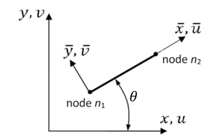
The local reference frame is $(\bar{x},\bar{y})$ . The $\bar{x}$ axis coincides with the neutral axis of the beam, while $\bar{y}$ is a principal axis of the cross-section.

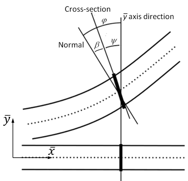
Two-node beam element with global and local coordinate systems and displacement components — Figure 1. Global and local coordinate systems and positive element displacement components.

Timoshenko beam cross-section showing the normal, the cross-section, and their rotations — Figure 2. Timoshenko kinematic quantities at a cross-section: normal rotation φ, cross-section rotation ψ, and shear angle β.

Each node has three degrees of freedom: the local displacements $\bar u,\bar v$ (or $u,v$ in the global frame) and the rotation $\psi$ of the cross-section.

The beam equations in the local reference frame are:

\left\{\begin{aligned}\frac{d\psi}{d\bar{x}}&=\frac{M}{EI}\\[4pt]\beta&=\frac{T}{GA_0}\\[4pt]\varphi&=\frac{d\bar v}{d\bar{x}}\\[4pt]\varphi&=\psi+\beta\end{aligned}\right.

The notation is retained exactly: $\varphi$ is the rotation of the normal, $\psi$ is the rotation of the cross-section, and the shear angle is:

\beta=\varphi-\psi

For the Timoshenko beam model, the angular nodal degree of freedom is $\psi$ , the rotation of the cross-section, not $\varphi$ , the rotation of the normal.

With the natural coordinate $\xi\in[-1,1]$ , the local coordinate, linear shape functions, and displacement interpolation are:

h_1(\xi)=\frac{1-\xi}{2},\qquad h_2(\xi)=\frac{1+\xi}{2},\qquad \bar x=h_1\bar x_1+h_2\bar x_2

\bar u=h_1\bar u_1+h_2\bar u_2,\qquad \bar v=h_1\bar v_1+h_2\bar v_2,\qquad \psi=h_1\psi_1+h_2\psi_2

Generalized strains and stresses

The generalized strains are the axial strain of the central fibre, the shear angle, and the curvature:

\varepsilon_0=\frac{d\bar u}{d\bar x},\qquad \beta=\frac{d\bar v}{d\bar x}-\psi,\qquad \kappa=\frac{d\psi}{d\bar x}

For the local element displacement vector:

\bar{\boldsymbol u}_{el}=\begin{Bmatrix}\bar u_1\\[3pt]\bar v_1\\[3pt]\psi_1\\[3pt]\bar u_2\\[3pt]\bar v_2\\[3pt]\psi_2\end{Bmatrix}

the individual strain-displacement relations are:

\varepsilon_0=\frac{d\bar u}{d\bar x}=\left[-1/L,\ 0,\ 0,\ 1/L,\ 0,\ 0\right]\bar{\boldsymbol u}_{el}=\boldsymbol B_{\varepsilon}\bar{\boldsymbol u}_{el}

\beta=\varphi-\psi=\left[0,\ -1/L,\ -h_1(\xi),\ 0,\ 1/L,\ -h_2(\xi)\right]\bar{\boldsymbol u}_{el}=\boldsymbol B_{\beta}\bar{\boldsymbol u}_{el}

\kappa=\left[0,\ 0,\ -1/L,\ 0,\ 0,\ 1/L\right]\bar{\boldsymbol u}_{el}=\boldsymbol B_{\kappa}\bar{\boldsymbol u}_{el}

\boldsymbol{\varepsilon}=\begin{Bmatrix}\varepsilon_0\\[3pt]\beta\\[3pt]\kappa\end{Bmatrix}=\begin{bmatrix}\boldsymbol B_{\varepsilon}\\[4pt]\boldsymbol B_{\beta}\\[4pt]\boldsymbol B_{\kappa}\end{bmatrix}\bar{\boldsymbol u}_{el}=\boldsymbol B\bar{\boldsymbol u}_{el}

\boldsymbol B=\begin{bmatrix}-1/L&0&0&1/L&0&0\\[6pt]0&-1/L&-h_1(\xi)&0&1/L&-h_2(\xi)\\[6pt]0&0&-1/L&0&0&1/L\end{bmatrix}

The derivatives with respect to the local coordinate follow from the chain rule:

\frac{d\bar v}{d\bar x}=\frac{d\bar v}{d\xi}\frac{d\xi}{d\bar x},\qquad \frac{d\xi}{d\bar x}=\left(\frac{d\bar x}{d\xi}\right)^{-1}=\left(\frac{-\bar x_1+\bar x_2}{2}\right)^{-1}=\frac{2}{L}

Hooke's law for the generalized strains and work-conjugate generalized stresses is:

\boldsymbol{\sigma}=\boldsymbol D\boldsymbol{\varepsilon},\qquad \begin{Bmatrix}N\\[3pt]T\\[3pt]M\end{Bmatrix}=\begin{bmatrix}EA&0&0\\[4pt]0&GA_0&0\\[4pt]0&0&EI\end{bmatrix}\begin{Bmatrix}\varepsilon_0\\[3pt]\beta\\[3pt]\kappa\end{Bmatrix}

\boldsymbol{\varepsilon}=\begin{Bmatrix}\varepsilon_0\\[3pt]\beta\\[3pt]\kappa\end{Bmatrix},\qquad \boldsymbol{\sigma}=\begin{Bmatrix}N\\[3pt]T\\[3pt]M\end{Bmatrix},\qquad \boldsymbol D=\begin{bmatrix}EA&0&0\\[4pt]0&GA_0&0\\[4pt]0&0&EI\end{bmatrix}

Here N, T, and M are the axial force, shear force, and bending moment. E and G are Young's modulus and the shear modulus; A, $A_0$ , and I are the cross-sectional area, effective shear area, and second moment of area.

Stiffness matrices

The element stiffness matrix in the local frame is [2]

\displaystyle \bar{\boldsymbol k}_{el}=\int_{-L/2}^{L/2}\boldsymbol B^{T}\boldsymbol D\boldsymbol B\,d\bar x=\frac{L}{2}\int_{-1}^{1}\boldsymbol B^{T}\boldsymbol D\boldsymbol B\,d\xi

Exact integration gives:

\bar{\boldsymbol k}_{el}^{A}=\frac{EA}{L}\begin{bmatrix}1&0&0&-1&0&0\\[3pt]0&0&0&0&0&0\\[3pt]0&0&0&0&0&0\\[3pt]-1&0&0&1&0&0\\[3pt]0&0&0&0&0&0\\[3pt]0&0&0&0&0&0\end{bmatrix}+\frac{GA_0}{L}\begin{bmatrix}0&0&0&0&0&0\\[3pt]0&1&L/2&0&-1&L/2\\[3pt]0&L/2&L^2/3&0&-L/2&L^2/6\\[3pt]0&0&0&0&0&0\\[3pt]0&-1&-L/2&0&1&-L/2\\[3pt]0&L/2&L^2/6&0&-L/2&L^2/3\end{bmatrix}+\frac{EI}{L}\begin{bmatrix}0&0&0&0&0&0\\[3pt]0&0&0&0&0&0\\[3pt]0&0&1&0&0&-1\\[3pt]0&0&0&0&0&0\\[3pt]0&0&0&0&0&0\\[3pt]0&0&-1&0&0&1\end{bmatrix}

Because the displacement and rotation interpolations are linear, exact integration produces shear locking and makes a slender beam artificially stiff. Better results are obtained with one-point Gauss integration at $\xi=0$ :

\displaystyle \bar{\boldsymbol k}_{el}^{B}=\frac{L}{2}\int_{-1}^{1}\boldsymbol B^{T}\boldsymbol D\boldsymbol B\,d\xi\approx L\boldsymbol B(0)^{T}\boldsymbol D\boldsymbol B(0)=L\left(EA\boldsymbol B_{\varepsilon}^{T}\boldsymbol B_{\varepsilon}+GA_0\boldsymbol B_{\beta}^{T}\boldsymbol B_{\beta}+EI\boldsymbol B_{\kappa}^{T}\boldsymbol B_{\kappa}\right)_{\xi=0}

\bar{\boldsymbol k}_{el}^{B}=\frac{EA}{L}\begin{bmatrix}1&0&0&-1&0&0\\[3pt]0&0&0&0&0&0\\[3pt]0&0&0&0&0&0\\[3pt]-1&0&0&1&0&0\\[3pt]0&0&0&0&0&0\\[3pt]0&0&0&0&0&0\end{bmatrix}+\frac{GA_0}{L}\begin{bmatrix}0&0&0&0&0&0\\[3pt]0&1&L/2&0&-1&L/2\\[3pt]0&L/2&L^2/4&0&-L/2&L^2/4\\[3pt]0&0&0&0&0&0\\[3pt]0&-1&-L/2&0&1&-L/2\\[3pt]0&L/2&L^2/4&0&-L/2&L^2/4\end{bmatrix}+\frac{EI}{L}\begin{bmatrix}0&0&0&0&0&0\\[3pt]0&0&0&0&0&0\\[3pt]0&0&1&0&0&-1\\[3pt]0&0&0&0&0&0\\[3pt]0&0&0&0&0&0\\[3pt]0&0&-1&0&0&1\end{bmatrix}

Shear locking and correction

If we modify the above last expression like this:

\bar{\boldsymbol k}_{el}^{C}=L\left(EA\boldsymbol B_{\varepsilon}^{T}\boldsymbol B_{\varepsilon}+\gamma GA_0\boldsymbol B_{\beta}^{T}\boldsymbol B_{\beta}+EI\boldsymbol B_{\kappa}^{T}\boldsymbol B_{\kappa}\right)_{\xi=0}

\bar{\boldsymbol k}_{el}^{C}=\frac{EA}{L}\begin{bmatrix}1&0&0&-1&0&0\\[3pt]0&0&0&0&0&0\\[3pt]0&0&0&0&0&0\\[3pt]-1&0&0&1&0&0\\[3pt]0&0&0&0&0&0\\[3pt]0&0&0&0&0&0\end{bmatrix}+\gamma\frac{GA_0}{L}\begin{bmatrix}0&0&0&0&0&0\\[3pt]0&1&L/2&0&-1&L/2\\[3pt]0&L/2&L^2/4&0&-L/2&L^2/4\\[3pt]0&0&0&0&0&0\\[3pt]0&-1&-L/2&0&1&-L/2\\[3pt]0&L/2&L^2/4&0&-L/2&L^2/4\end{bmatrix}+\frac{EI}{L}\begin{bmatrix}0&0&0&0&0&0\\[3pt]0&0&0&0&0&0\\[3pt]0&0&1&0&0&-1\\[3pt]0&0&0&0&0&0\\[3pt]0&0&0&0&0&0\\[3pt]0&0&-1&0&0&1\end{bmatrix}

m=\frac{12EI}{L^2GA_0},\qquad \gamma=\frac{m}{1+m}

The factor $\gamma$ scales the one-point shear contribution according to the bending-to-shear stiffness ratio. It is a dimensionless correction; no additional derivation is required for its use here.

Using one-point Gauss integration together with the correction factor $\gamma$ , the stiffness matrix becomes identical to the expression obtained for the Timoshenko beam element presented in Section 5.2. This equality holds although Section 5.2 uses a cubic interpolation for the transverse displacement $\bar v$ .

Numerical examples

Example 1. Consider a cantilever with $L=100\ \mathrm{mm}$ , $E=2\times10^5\ \mathrm{MPa}$ , $G=E/2.5$ , and rectangular cross-section $5\ \mathrm{mm}\times20\ \mathrm{mm}$ . The force $F=10^4\ \mathrm{N}$ is applied at the free end, perpendicular to the undeformed beam axis; the axial force is $H=35\ \mathrm{N}$ .

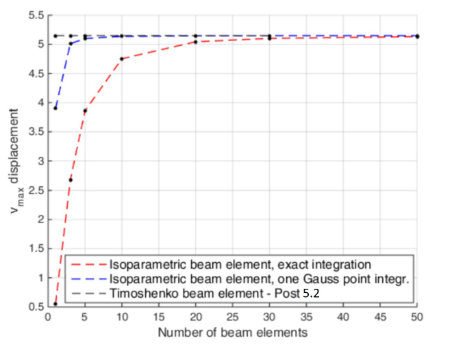
The exactly integrated element $\bar{\boldsymbol k}_{el}^{A}$ converges only for a relatively large number of elements. The one-point element $\bar{\boldsymbol k}_{el}^{B}$ converges much faster, while the corrected element $\bar{\boldsymbol k}_{el}^{C}$ gives the Section 5.2 result for any mesh.

Free-end displacement versus number of beam elements for three Timoshenko formulations — Figure 3. Free-end vertical displacement versus the number of beam elements. Exact integration exhibits shear locking; one-point integration converges much faster, and the corrected formulation reproduces the Section 5.2 result.

Example 2. For the same cantilever and cross-section under the end couple $C=10^6\ \mathrm{N\,mm}$ , the loading is pure bending and the physical shear force is zero. With three exactly integrated elements, $\bar{\boldsymbol k}_{el}^{A}$ gives $v_{max}=3.89\ \mathrm{mm}$ instead of the correct value

v_{max}=\frac{CL^2}{2EI}=7.5\ \mathrm{mm}

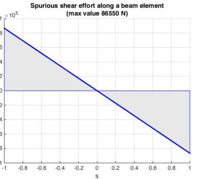
The excessive stiffness is caused by a spurious shear force that varies linearly within each element. Its average resultant contribution over the finite element is zero, and it is also zero at the element midpoint $\xi=0$ . One-point Gauss integration samples this midpoint and therefore eliminates the spurious shear contribution in pure bending. Consequently, $\bar{\boldsymbol k}_{el}^{B}$ gives zero shear force and the exact displacement $v_{max}=7.5\ \mathrm{mm}$ .

Spurious shear force along an exactly integrated beam element in pure bending — Figure 4. Spurious shear force along an exactly integrated isoparametric beam element in the pure-bending example.

MATLAB programs

The package contains four commented files. gen.m defines the model; stiff.m assembles the corrected one-point element; stress.m recovers N, T, and M; and main.m runs the analysis and plots the results.

stiff.mCorrected one-point integration

%*** stiff.m ***
gamma = 12*ei/(L^2*ga + 12*ei);
gac = gamma*ga;
% One-point shear contribution with correction
K(ip,ip) = K(ip,ip) + R'*kel*R;

MATLAB compatibility

Tested in MATLAB R2024a. The code uses standard MATLAB syntax and is expected to be compatible with newer MATLAB versions. No additional toolbox is required.

MIsoparametric Timoshenko beam MATLAB package4 commented MATLAB files and README · tested in R2024aDownload ZIP

References

O. C. Zienkiewicz, R. L. Taylor, and J. Z. Zhu, The Finite Element Method: Its Basis and Fundamentals, 7th ed., Elsevier, 2013.
K. J. Bathe, Finite Element Procedures, 2nd ed., Klaus-Jürgen Bathe, 2014.