6. Beam Finite Element — Nonlinear Double-Clamped Beam

Model and constitutive relations

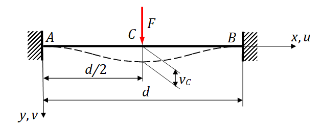
A double-clamped beam is loaded at its midpoint by the force $F$ [2].

MaterialLinear elastic

StrainSmall

DisplacementModerately large

Double-clamped beam of span d with a midpoint force F and midpoint displacement v sub C — Figure 1. Double-clamped beam, geometry, load, and displacement notation.

Points $A$ and $B$ are completely fixed. Because the axial displacements of both ends are restrained, an axial force develops as the beam deflects.

\left\{\begin{array}{c}u_A=0\\[4pt]v_A=0\\[4pt]\varphi_A=0\end{array}\right.

\left\{\begin{array}{c}u_B=0\\[4pt]v_B=0\\[4pt]\varphi_B=0\end{array}\right.

The displacement-dependent axial strain makes the problem nonlinear. For the Euler–Bernoulli beam model, the generalized strain and work-conjugate generalized stress vectors are:

\boldsymbol{\varepsilon}=\left\{\begin{array}{c}\varepsilon_0\\[4pt]\kappa\end{array}\right\},\qquad \boldsymbol{\sigma}=\left\{\begin{array}{c}N\\[4pt]M\end{array}\right\}

In this planar analysis, $T$ and $T_y$ denote the same transverse force component, while $M$ and $M_z$ denote the same bending moment component.

Hooke's law is:

\boldsymbol{\sigma}=\boldsymbol D\boldsymbol{\varepsilon},\qquad \boldsymbol D=\left[\begin{array}{cc}EA&0\\[4pt]0&EI\end{array}\right]

or, component by component,

N=EA\varepsilon_0,\qquad M=EI\kappa

$\varepsilon_0$: axial strain of the neutral axis
$\kappa$: curvature of the neutral axis
$N$: axial force
$M$: bending moment
$E$: Young's modulus
$A,\ I$: cross-sectional area and second moment of area

Cubic beam finite element

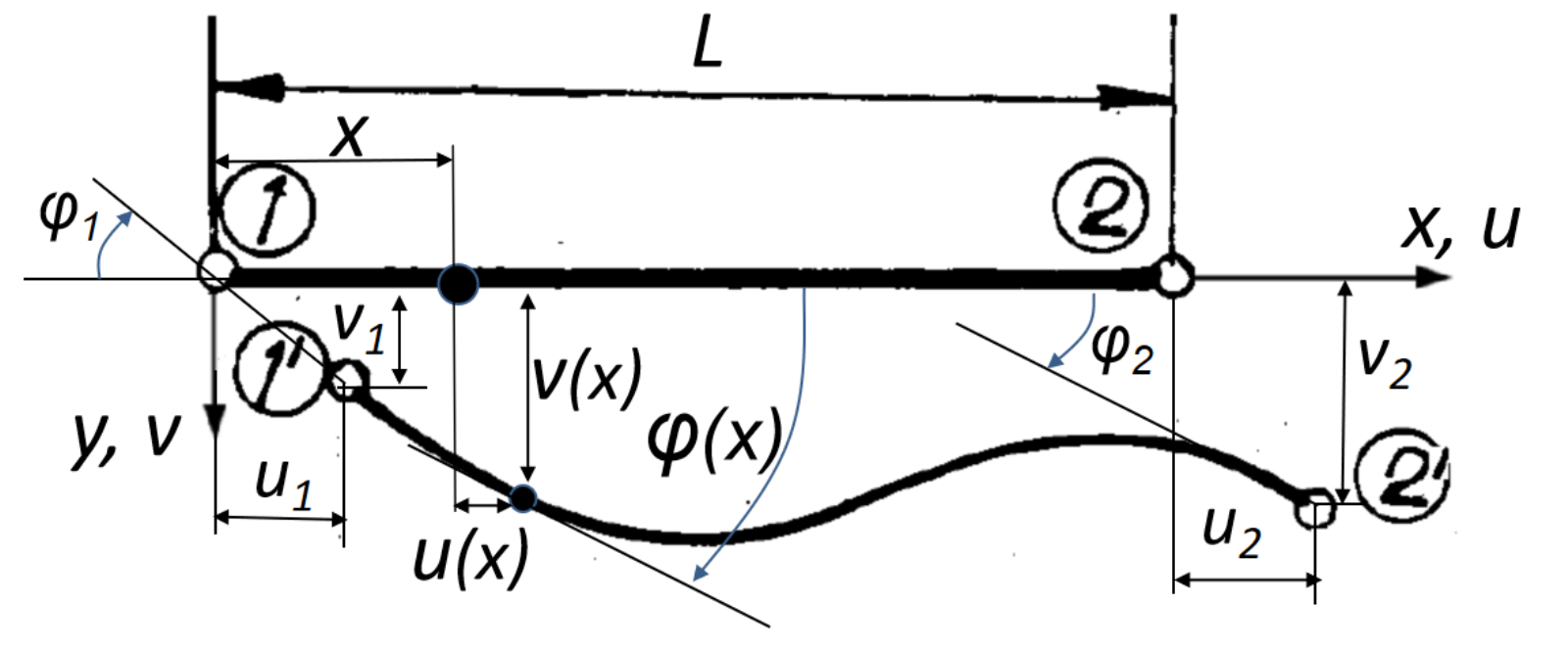
Cubic two-node beam finite element with nodal axial and transverse displacements and rotations — Figure 2. Two-node cubic beam finite element and its six nodal degrees of freedom.

With the normalized coordinate $\xi=x/L$ , the axial displacement is interpolated linearly and the transverse displacement cubically. These are the standard Euler–Bernoulli interpolation functions used in Section 5.1 [1].

u(x)=\left[1-\xi,\ 0,\ 0,\ \xi,\ 0,\ 0\right]\boldsymbol u_{el}=\boldsymbol N_u\boldsymbol u_{el}

v(x)=\left[0,\ 2\xi^3-3\xi^2+1,\ (\xi^3-2\xi^2+\xi)L,\ 0,\ -2\xi^3+3\xi^2,\ (\xi^3-\xi^2)L\right]\boldsymbol u_{el}=\boldsymbol N_v\boldsymbol u_{el}

\varphi(x)=\frac{dv}{dx}=\left[0,\ \frac{6\xi^2-6\xi}{L},\ 3\xi^2-4\xi+1,\ 0,\ \frac{-6\xi^2+6\xi}{L},\ 3\xi^2-2\xi\right]\boldsymbol u_{el}=\boldsymbol N_{v,x}\boldsymbol u_{el}

\boldsymbol u_{el}=\left\{\begin{array}{c}u_1\\[3pt]v_1\\[3pt]\varphi_1\\[3pt]u_2\\[3pt]v_2\\[3pt]\varphi_2\end{array}\right\}

Here $L$ is the element length and $\boldsymbol u_{el}$ is the element nodal-displacement vector.

Moderately large-displacement strain

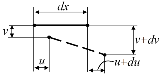
Differential neutral-axis segment before and after axial and transverse displacement — Figure 3. Differential geometry used to derive the axial strain.

The exact axial strain of the neutral axis obtained from Figure 3 is:

\varepsilon_0=\frac{\sqrt{(dx+du)^2+dv^2}-dx}{dx}=\sqrt{\left(1+\frac{du}{dx}\right)^2+\left(\frac{dv}{dx}\right)^2}-1

\varepsilon_0=\sqrt{1+2\frac{du}{dx}+\left(\frac{du}{dx}\right)^2+\left(\frac{dv}{dx}\right)^2}-1

The square root is expanded as:

\sqrt{1+a}\approx1+\frac12a-\frac18a^2,\qquad a=2\frac{du}{dx}+\left(\frac{du}{dx}\right)^2+\left(\frac{dv}{dx}\right)^2

After terms of third or higher degree are neglected, the moderately large-displacement approximation is:

\varepsilon_0\approx\frac{du}{dx}+\frac12\left(\frac{dv}{dx}\right)^2

The generalized strain vector is therefore:

\boldsymbol{\varepsilon}=\left\{\begin{array}{c}\varepsilon_0\\[5pt]\kappa\end{array}\right\}=\left\{\begin{array}{c}\dfrac{du}{dx}+\dfrac12\left(\dfrac{dv}{dx}\right)^2\\[10pt]\dfrac{d^2v}{dx^2}\end{array}\right\}

The derivatives of the interpolation functions are:

\frac{du}{dx}=\frac1L\left[-1,\ 0,\ 0,\ 1,\ 0,\ 0\right]\boldsymbol u_{el}=\boldsymbol N_{u,x}\boldsymbol u_{el}

\frac{dv}{dx}=\left[0,\ \frac{6\xi^2-6\xi}{L},\ 3\xi^2-4\xi+1,\ 0,\ \frac{-6\xi^2+6\xi}{L},\ 3\xi^2-2\xi\right]\boldsymbol u_{el}=\boldsymbol N_{v,x}\boldsymbol u_{el}

\kappa=\frac{d^2v}{dx^2}=\left[0,\ \frac{12\xi-6}{L^2},\ \frac{6\xi-4}{L},\ 0,\ \frac{-12\xi+6}{L^2},\ \frac{6\xi-2}{L}\right]\boldsymbol u_{el}=\boldsymbol N_{\kappa}\boldsymbol u_{el}

Hence,

\varepsilon_0=\boldsymbol N_{u,x}\boldsymbol u_{el}+\frac12\left(\boldsymbol N_{v,x}\boldsymbol u_{el}\right)^2,\qquad \kappa=\boldsymbol N_{\kappa}\boldsymbol u_{el}

Potential energy and nonlinear equilibrium

The total potential energy, summed over all beam elements, is:

\Pi=\underbrace{\frac12\sum_{el}\int_0^L\boldsymbol{\varepsilon}^{T}\boldsymbol D\boldsymbol{\varepsilon}\,dx}_{U}\;\underbrace{-\boldsymbol u^{T}\boldsymbol F}_{V}

\Pi=\underbrace{\frac12\sum_{el}\int_0^L\left(EA\varepsilon_0^2+EI\kappa^2\right)dx}_{U}\;\underbrace{-\boldsymbol u^{T}\boldsymbol F}_{V}

$U$ is the deformation energy, $V$ is the potential of the external nodal-force vector $\boldsymbol F$ , and $\boldsymbol u$ is the assembled nodal-displacement vector.

The minimum-total-potential-energy condition is:

\boldsymbol\Psi=\frac{\partial\Pi}{\partial\boldsymbol u}=\boldsymbol0

This condition produces the nonlinear algebraic system $\boldsymbol\Psi(\boldsymbol u)=\boldsymbol0$ . At iteration $i$ , the Newton–Raphson update is:

\Delta\boldsymbol u^{(i)}=-\left[\boldsymbol K_t\!\left(\boldsymbol u^{(i)}\right)\right]^{-1}\boldsymbol\Psi\!\left(\boldsymbol u^{(i)}\right)

\boldsymbol u^{(i+1)}=\boldsymbol u^{(i)}+\Delta\boldsymbol u^{(i)}

The residual and tangent stiffness are:

\boldsymbol\Psi=\frac{\partial U}{\partial\boldsymbol u}-\boldsymbol F=\sum_{el}\boldsymbol f_{el}-\boldsymbol F

\boldsymbol K_t(\boldsymbol u)=\frac{\partial^2U}{\partial\boldsymbol u^2}=\sum_{el}\frac{\partial^2U_{el}}{\partial\boldsymbol u_{el}^2}=\sum_{el}\boldsymbol k_{el}

Element residual and tangent stiffness

The deformation energy of one finite element is:

U_{el}=\frac12\int_0^L\boldsymbol{\varepsilon}^{T}\boldsymbol D\boldsymbol{\varepsilon}\,dx=\frac12\int_0^L\left(EA\varepsilon_0^2+EI\kappa^2\right)dx

Using Gaussian quadrature,

U_{el}=\frac12\sum_{G=1}^{n_G}\eta_G\left(EA\varepsilon_{0G}^{2}+EI\kappa_G^{2}\right)\frac L2,\qquad \varepsilon_{0G}=\varepsilon_0(\xi_G),\quad \kappa_G=\kappa(\xi_G)

Two Gauss points are sufficient, $n_G=2$ . On $0\leq\xi\leq1$ , their coordinates and weights are:

\xi_G=\frac12\left(1\pm\frac{\sqrt3}{3}\right),\qquad \eta_G=1

The element unbalanced-force vector and tangent stiffness matrix follow by differentiation:

\boldsymbol f_{el}=\frac{\partial U_{el}}{\partial\boldsymbol u_{el}},\qquad \boldsymbol k_{el}=\frac{\partial\boldsymbol f_{el}}{\partial\boldsymbol u_{el}}=\frac{\partial^2U_{el}}{\partial\boldsymbol u_{el}^2}

\boldsymbol f_{el}=\sum_{G=1}^{2}\left(EA\varepsilon_0\frac{\partial\varepsilon_0}{\partial\boldsymbol u_{el}}+EI\kappa\frac{\partial\kappa}{\partial\boldsymbol u_{el}}\right)_G\frac L2

\boldsymbol k_{el}=\sum_{G=1}^{2}\left[EA\varepsilon_0\frac{\partial^2\varepsilon_0}{\partial\boldsymbol u_{el}^2}+EA\frac{\partial\varepsilon_0}{\partial\boldsymbol u_{el}}\left(\frac{\partial\varepsilon_0}{\partial\boldsymbol u_{el}}\right)^T+EI\kappa\frac{\partial^2\kappa}{\partial\boldsymbol u_{el}^2}+EI\frac{\partial\kappa}{\partial\boldsymbol u_{el}}\left(\frac{\partial\kappa}{\partial\boldsymbol u_{el}}\right)^T\right]_G\frac L2

The required first and second derivatives are:

\frac{\partial\varepsilon_0}{\partial\boldsymbol u_{el}}=\boldsymbol N_{u,x}^{T}+\left(\boldsymbol N_{v,x}^{T}\boldsymbol N_{v,x}\right)\boldsymbol u_{el},\qquad \frac{\partial\kappa}{\partial\boldsymbol u_{el}}=\boldsymbol N_{\kappa}^{T}

\frac{\partial^2\varepsilon_0}{\partial\boldsymbol u_{el}^2}=\boldsymbol N_{v,x}^{T}\boldsymbol N_{v,x},\qquad \frac{\partial^2\kappa}{\partial\boldsymbol u_{el}^2}=\boldsymbol0_{6\times6}

Element vectors and matrices are assembled in the standard way:

\boldsymbol\Psi=\sum_{el}\boldsymbol f_{el}-\boldsymbol F,\qquad \boldsymbol K_t=\sum_{el}\boldsymbol k_{el}=\sum_{el}\frac{\partial\boldsymbol f_{el}}{\partial\boldsymbol u_{el}}

The iterative process stops when the displacement-correction norm is smaller than the prescribed tolerance.

Example 1 — double-clamped beam

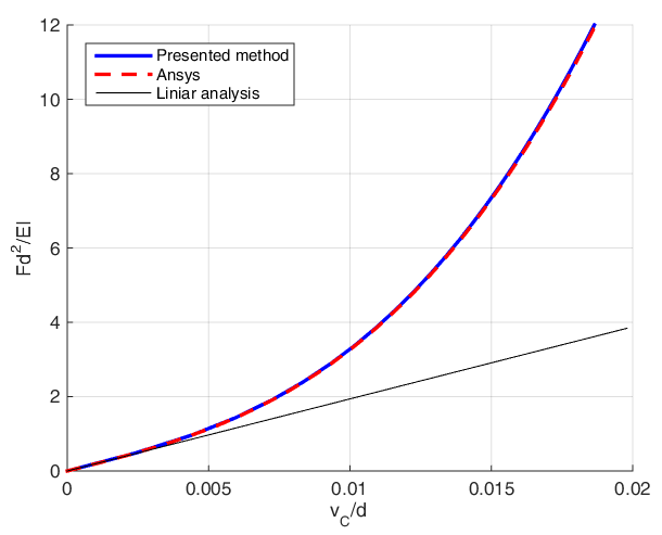
The beam has a rectangular cross-section $w\times t=5\ \mathrm{mm}\times1\ \mathrm{mm}$ , span $d=100\ \mathrm{mm}$ , Young's modulus $E=2\times10^5\ \mathrm{MPa}$ , and midpoint force $F=100\ \mathrm N$ . The MATLAB result agrees with the ANSYS large-deformation model. At the final load step,

v_C=-1.86555\ \mathrm{mm},\qquad \frac{|v_C|}{d}=0.0186555,\qquad \frac NF=8.01210

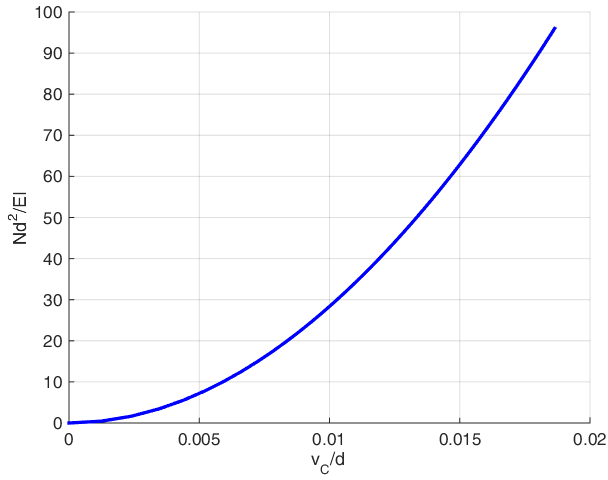
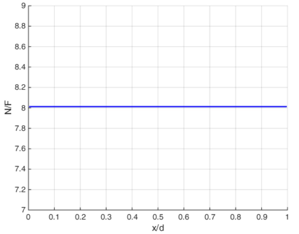
Although $|v_C|/d<0.02$ , the difference from the linear response is clearly visible. The axial force induced by the two axial restraints is constant along the beam.

Dimensionless force versus midpoint displacement, comparing the presented method, ANSYS, and linear analysis — Figure 4. Force versus midpoint displacement. The MATLAB and ANSYS curves coincide; the linear response is also shown.

Dimensionless axial force versus midpoint displacement — Figure 5. Axial force versus midpoint displacement. The axial force is constant along the beam at every load step.

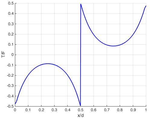
Normalized shear-force diagram at 100 newtons — Figure 6. Shear-force diagram for $F=100\ \mathrm N$ .

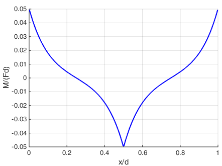
Normalized bending-moment diagram at 100 newtons — Figure 7. Bending-moment diagram for $F=100\ \mathrm N$ .

Constant normalized axial force along the double-clamped beam — Figure 8. Constant axial-force ratio along the beam: $N/F=8.012$ .

Example 2 — cantilever

Consider a cantilever with $w\times t=5\ \mathrm{mm}\times1\ \mathrm{mm}$ , $L=100\ \mathrm{mm}$ , $E=2\times10^5\ \mathrm{MPa}$ , and a transverse free-end force $F=4\ \mathrm N$ . The normalized maximum displacement is:

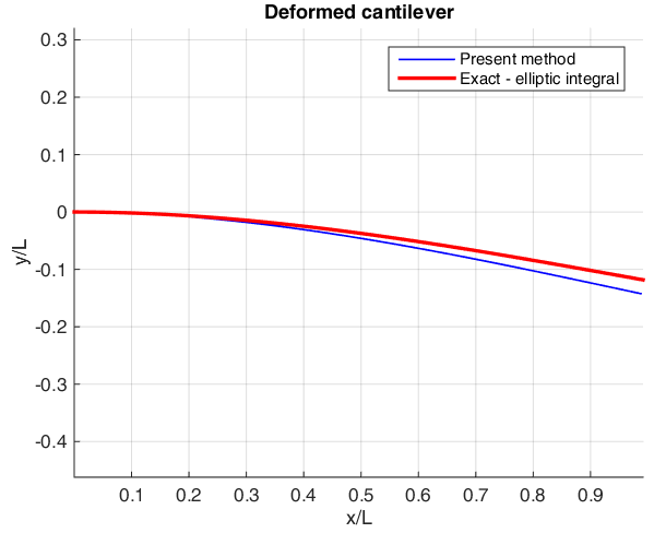
\begin{aligned}\text{linear model:}\quad &\frac{v_{max}}L=\frac{FL^2}{3EI}=0.160\\[5pt]\text{presented method, 40 elements:}\quad &\frac{v_{max}}L=0.1424\\[5pt]\text{exact elastica:}\quad &\frac{v_{max}}L=0.1183\end{aligned}

The error of the moderately large-displacement approximation relative to the exact elastica result is about 20%. The approximation is suitable when the slope $\varphi$ is less than approximately $10^\circ\approx0.175\ \mathrm{rad}$ , for which

\varphi^2=\left(\frac{dv}{dx}\right)^2\approx0.03

This term is then small compared with unity [2]. In the present example, $\varphi_{max}\approx0.21\ \mathrm{rad}\approx12^\circ$ .

Deformed cantilever comparison between the presented method and exact elastica — Figure 9. Deformed cantilever: moderately large-displacement approximation and exact elastica.

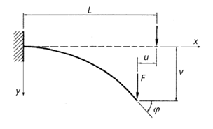
Cantilever geometry with free-end displacement and rotation — Figure 10. Cantilever load, displacement, and rotation notation.

MATLAB and ANSYS files

The MATLAB package contains the complete nonlinear analysis, result recovery, diagram generation, and a README. The code follows the element equations above: deriv.m evaluates $\varepsilon_0$ , $\kappa$ , and their derivatives; stiff.m integrates and assembles $\boldsymbol f_{el}$ and $\boldsymbol k_{el}$ ; and main.m performs the load-step and Newton–Raphson loops.

deriv.mStrain and curvature

%*** deriv ***
ep = Nux*uel + 1/2*(Nvx*uel)^2;
ep1 = Nux' + (Nvx'*Nvx)*uel;
ep2 = Nvx'*Nvx;

ka = Nka*uel;
ka1 = Nka';

MATLAB compatibility

Tested in MATLAB R2024a. The code uses standard MATLAB syntax and is expected to be compatible with newer MATLAB versions. No additional toolbox is required.

MNonlinear beam MATLAB package7 commented MATLAB files and README · tested in R2024aDownload ZIP AANSYS verification packageMechanical APDL half-beam model and READMEDownload ZIP

The ANSYS macro uses symmetry: it models half of the beam, imposes the midpoint symmetry conditions, and applies $F/2=50\ \mathrm N$ to represent the $100\ \mathrm N$ force on the complete beam. The macro was inspected against the model definition; ANSYS was not available in the local execution environment.

References

C. A. Felippa, Introduction to Finite Element Methods.
Massachusetts Institute of Technology, Lecture 6: Moderately Large Deflection Theory of Beams, Structural Mechanics, 2013.