01
Purpose and benchmark model
triang2d_fast is a high-speed implementation of the constant-strain triangular solver used in Section 9.1. Its principal acceleration comes from evaluating the element matrices for all finite elements simultaneously and from vectorized sparse assembly.
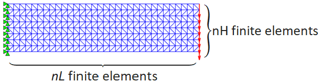
The benchmark uses the same rectangular plane-stress cantilever for both implementations. The mesh has subdivisions through the height and subdivisions along the length, giving
02
Simultaneous element computations
For finite elements, the strain-displacement and constitutive matrices are stored as three-dimensional arrays:
B(:,:,ie) is the strain-displacement matrix of element ie. DHooke(:,:,ie) is the corresponding plane-stress constitutive matrix multiplied by the element area and thickness. The function multiprod performs the products for all elements in one operation:
DBt=multiprod(DHooke,B);

kelt=reshape(multiprod(permute(B,[2 1 3]),DBt),36,nel);
DBt stores the products for all finite elements. These products are then used to compute the element stiffness matrices and remain available in element-wise form for the standard stress-postprocessing routine.
kelt has 36 rows and nel columns. Each column contains the 36 entries of the stiffness matrix of one finite element.
03
Vectorized sparse assembly
The arrays ipos1 and ipos2 contain the global row and column positions of every element-stiffness entry. neq is the total number of equations. MATLAB then assembles the global matrix in a single sparse-matrix construction:
ipos0=[ngn*nodo1-1 ngn*nodo1 ...
       ngn*nodo2-1 ngn*nodo2 ...
       ngn*nodo3-1 ngn*nodo3]';
ipos1=[ipos0; ipos0; ipos0; ipos0; ipos0; ipos0];
ipos2=permute(reshape(ipos1,6,6,nel),[2 1 3]);
K=sparse(ipos1,ipos2(:),kelt(:),neq,neq);
K is the global sparse stiffness matrix. This construction replaces the repeated element-by-element additions K(ip,ip)=K(ip,ip)+kel used by the standard solver.
04
Global system solution
After imposing the nodal loads and constraints, both implementations solve the same finite element system
In the MATLAB implementation, F is the global load vector and the solution is stored in the program variable S:
S=K\F;The backslash operation is common to the standard and fast solvers. The principal algorithmic difference lies before this solve, in element-matrix computation and global stiffness assembly.
05
Use with Section 9.1
Start from the complete MATLAB programs supplied in Section 9.1, add triang2d_fast.m and multiprod.m, and replace the call triang2d in main.m with triang2d_fast.
For compatibility with the standard stress-postprocessing routine, the vectorized solver provides DBt in element-wise form. Thus, the same plot_stress routine can be used independently of the internal assembly strategy.
06
MATLAB R2026a benchmark
Intel Core i7-14700 @ 2.10 GHz, 32 GB RAM, Windows 11, MATLAB R2026a.
Each published row is the arithmetic mean of three measured runs after one unrecorded warm-up run of each implementation. Both solvers used exactly the same physical model and mesh. The following intervals were measured directly:
- Total: the complete solver computation, including matrix construction, loads, constraints, and the linear equation solution .
- Element computation + assembly: element matrices and global sparse stiffness assembly; this interval is not inferred by subtraction.
K\F: the global linear-system solution. The table reports the directly measured value from the fast-solver runs.
The published assembly speed-up values use the directly measured assembly-stage times in this ratio; they were not obtained by subtracting the linear-system solution time from the total time.
For example, means that the complete measured computation is ten times faster with triang2d_fast.
| CST elements | Equations | Standardtotal (s) | Fasttotal (s) | Fast K\F(s) | Overallspeed-up | Standardassembly (s) | Fastassembly (s) | Assemblyspeed-up | |
|---|---|---|---|---|---|---|---|---|---|
| 80 × 200 | 32,000 | 32,562 | 34.378 | 0.220 | 0.126 | 156.4× | 33.998 | 0.083 | 410.4× |
| 100 × 250 | 50,000 | 50,702 | 64.564 | 0.292 | 0.172 | 221.3× | 64.092 | 0.100 | 642.4× |
The current measurements show that vectorization and direct sparse assembly reduce the pre-solve stage by more than two orders of magnitude for both meshes. The complete-computation acceleration is smaller because K\F is common to both algorithms and therefore represents a larger fraction of the fast solver's total time.
For a much larger mesh with and , corresponding to 1,253,502 global equations, triang2d_fast required 2.553 s for element-matrix generation and assembly, while the solution of the global linear system required 21.487 s. This case illustrates how, once assembly becomes extremely efficient, solution of the global sparse linear system becomes the dominant part of the computation.
07
Numerical equivalence
Before the timings were accepted, the global displacement vectors and the element stress fields produced by the two implementations were compared for every benchmark mesh.
| Absolute displacement difference | Relative displacement difference | Absolute stress difference | Relative stress difference | |
|---|---|---|---|---|
| 80 × 200 | ||||
| 100 × 250 |
The differences are at floating-point round-off level for these computations. No material difference was found in representative nodal displacements, displacement extrema, or element stress extrema.
08
Programs and downloads
The standard and fast solvers were executed in MATLAB R2026a on both published benchmark meshes. The package contains the fast routine, multiprod, its BSD license, and a README.
multiprod.m is by Paolo de Leva and is redistributed under the included BSD-style license. Its authoritative distribution page is the MATLAB Central File Exchange entry.