01
Purpose and strategy
triang2d_fast2 is an alternative high-speed implementation of the CST solver presented in Section 9.1. It is intended for users who wish to avoid the external multiprod function employed by Section 9.2.
Section 9.2 stores the element matrices in three-dimensional arrays and performs the batched products with multiprod. The present routine instead places every element matrix in a large two-dimensional block-diagonal sparse matrix. Standard sparse matrix multiplication then evaluates the products corresponding to for all elements.
02
Block-diagonal sparse matrices
For a mesh containing constant-strain triangles, the matrices have dimensions
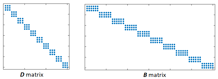
Each element strain-displacement matrix has dimensions , while each plane-stress constitutive block has dimensions . These blocks are placed on the diagonals of the large sparse matrices:
03
Sparse multiplication and assembly
The matrices and are assembled as large sparse block-diagonal matrices. Their standard matrix product provides the element stiffness contributions, while MATLAB sparse is then used for the global assembly.
DB=DHooke*B;
kelt=B'*DB;
DB contains the products in block-diagonal form, and kelt contains the corresponding element stiffness matrices. The index vector ij extracts their 36 entries per element, while ipos1 and ipos2 identify the associated global equation positions:
ij=(ip1(:)-1)*ngel*nel+ip2(:);
K=sparse(ipos1(:),ipos2(:),kelt(ij),neq,neq);
neq is the number of global equations. After the loads and constraints are imposed, K is the global stiffness matrix, F is the global load vector, and the MATLAB displacement variable S is obtained from
S=K\F;After the solution, the block-sparse product is converted to the element-wise array required by the standard stress-postprocessing routine:
% Convert DB for use with standard plot_stress postprocessing
ii=reshape(1:3*nel,3,1,nel)+(reshape(1:6*nel,1,6,nel)-1)*3*nel;
DBt=reshape(full(DB(ii(:))),3,6,nel);
DBt = DBt./reshape(Ath,1,1,[]);
04
Use with Section 9.1
Start from the MATLAB programs provided in Section 9.1, add triang2d_fast2.m, and replace the call triang2d in main.m with triang2d_fast2. The alternative package therefore contains only the new routine and its README.
For compatibility with the standard stress-postprocessing routine, the vectorized solver also provides DBt in element-wise form. Thus, the same plot_stress routine can be used independently of the internal assembly strategy.
05
MATLAB R2026a benchmark
Intel Core i7-14700 @ 2.10 GHz, 32 GB RAM, Windows 11, MATLAB R2026a.
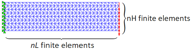
The two representative meshes are identical to those used in the current Section 9.2 benchmark. The Section 9.3 values are arithmetic means of three measured runs after one unrecorded warm-up run. Total time includes matrix construction, loads, constraints, and the solution ; assembly and linear-solve intervals were also measured directly.
| CST elements | Equations | 9.2total (s) | 9.3total (s) | 9.2assembly (s) | 9.3assembly (s) | 9.3 K\F(s) | |
|---|---|---|---|---|---|---|---|
| 80 × 200 | 32,000 | 32,562 | 0.220 | 0.160 | 0.083 | 0.093 | 0.061 |
| 100 × 250 | 50,000 | 50,702 | 0.292 | 0.305 | 0.100 | 0.169 | 0.093 |
The block-sparse alternative remains extremely fast, but its element-generation and assembly stage is slower than the multiprod implementation: approximately 1.13 times for the mesh and 1.69 times for the mesh. Total times are also influenced by run-to-run variation in the common sparse linear-system solution, so the directly measured assembly interval gives the clearest comparison of the two strategies.
For the larger mesh with and , corresponding to 1,253,502 global equations, the supplied triang2d_fast2 result is 4.924 s for element-matrix generation and assembly. The corresponding Section 9.2 value is 2.553 s. The alternative solver therefore remains very fast, while the multiprod formulation is faster at this stage.
06
Numerical equivalence
The global displacement vector and element stress field from triang2d_fast2 were compared with the Section 9.2 solver for both measured meshes.
| Maximum displacement difference | Relative displacement difference | Maximum stress difference | Relative stress difference | |
|---|---|---|---|---|
| 80 × 200 | 0 | 0 | 0 | 0 |
| 100 × 250 | 0 | 0 | 0 | 0 |
No numerical difference was recorded in the double-precision comparisons of nodal displacements, displacement extrema, or CST stress components.
07
Program download
triang2d_fast2 was executed in MATLAB R2026a on both published benchmark meshes. The routine requires the complete Section 9.1 package but has no external multiprod dependency.