9.1 CST Finite Element

CST element and hypotheses

The constant-strain triangle (CST) is a three-node finite element with two translational degrees of freedom at each node. The standard formulation introduced here follows the finite element treatment presented by Felippa [1].

StrainSmall

DisplacementSmall

MaterialLinear elastic

Stress statePlane stress

Element definition

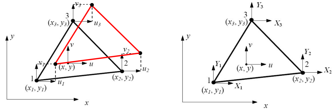
Three nodes; two translational degrees of freedom per node: $u_i$ and $v_i$ .

Three-node CST element showing nodal displacements, nodal forces, and global coordinates — **Figure 1.** Three-node CST element: nodal displacements and the corresponding nodal force components.

\boldsymbol{f}_{el}=\boldsymbol{k}_{el}\boldsymbol{u}_{el} \qquad \boldsymbol{u}_{el}= \begin{Bmatrix}u_1&v_1&u_2&v_2&u_3&v_3\end{Bmatrix}^{T} \qquad \boldsymbol{f}_{el}= \begin{Bmatrix}X_1&Y_1&X_2&Y_2&X_3&Y_3\end{Bmatrix}^{T}

Interpolation functions

The displacement field inside the element is interpolated from the six nodal displacement components:

\begin{Bmatrix}u(x,y)\\v(x,y)\end{Bmatrix} =\boldsymbol{N}\boldsymbol{u}_{el}

\boldsymbol{N}= \begin{bmatrix}\boldsymbol{N}_u\\\boldsymbol{N}_v\end{bmatrix} = \begin{bmatrix} N_1(x,y)&0&N_2(x,y)&0&N_3(x,y)&0\\ 0&N_1(x,y)&0&N_2(x,y)&0&N_3(x,y) \end{bmatrix}

N_1(x,y)=\frac{1}{2A_{el}} \left[(y_2-y_3)x-(x_2-x_3)y+x_2y_3-x_3y_2\right]

N_2(x,y)=\frac{1}{2A_{el}} \left[(y_3-y_1)x-(x_3-x_1)y+x_3y_1-x_1y_3\right]

N_3(x,y)=\frac{1}{2A_{el}} \left[(y_1-y_2)x-(x_1-x_2)y+x_1y_2-x_2y_1\right]

Strain-displacement matrix

Differentiation of the interpolation functions gives the constant strain-displacement matrix:

\boldsymbol{B}= \begin{bmatrix} \dfrac{\partial}{\partial x}&0\\[4pt] 0&\dfrac{\partial}{\partial y}\\[4pt] \dfrac{\partial}{\partial y}&\dfrac{\partial}{\partial x} \end{bmatrix} \begin{bmatrix}\boldsymbol{N}_u\\\boldsymbol{N}_v\end{bmatrix}

\boldsymbol{B}=\frac{1}{2A_{el}} \begin{bmatrix} y_2-y_3&0&y_3-y_1&0&y_1-y_2&0\\ 0&x_3-x_2&0&x_1-x_3&0&x_2-x_1\\ x_3-x_2&y_2-y_3&x_1-x_3&y_3-y_1&x_2-x_1&y_1-y_2 \end{bmatrix}

The signed element area used in these expressions is:

A_{el}=\frac{1}{2}\left[(x_2-x_1)(y_3-y_1)-(x_3-x_1)(y_2-y_1)\right]

Strains, stresses, and constitutive law

For plane stress, the strain and stress vectors and Hooke's law are:

\boldsymbol{\sigma}=\boldsymbol{D}\boldsymbol{\varepsilon} \qquad \boldsymbol{\sigma}=\begin{Bmatrix}\sigma_x\\\sigma_y\\\tau_{xy}\end{Bmatrix} \qquad \boldsymbol{\varepsilon}=\begin{Bmatrix}\varepsilon_x\\\varepsilon_y\\\gamma_{xy}\end{Bmatrix} =\boldsymbol{B}\boldsymbol{u}_{el}

\boldsymbol{D}=\frac{E}{1-\nu^2} \begin{bmatrix} 1&\nu&0\\ \nu&1&0\\ 0&0&\dfrac{1-\nu}{2} \end{bmatrix}

Here $E$ is Young's modulus and $\nu$ is Poisson's ratio.

Potential energy and virtual work

For an assemblage of finite elements, the total potential energy may be written in either of the equivalent forms. Here $\boldsymbol{u}$ is the global vector containing all nodal displacement degrees of freedom of the finite element discretization.

\Pi=\frac{1}{2}\sum_{el}\int_{V_{el}}\boldsymbol{\varepsilon}^{T}\boldsymbol{\sigma}\,dV -\boldsymbol{u}^{T}\boldsymbol{F}

\Pi=\frac{1}{2}\sum_{el}\int_{V_{el}}\boldsymbol{\varepsilon}^{T}\boldsymbol{D}\boldsymbol{\varepsilon}\,dV -\boldsymbol{u}^{T}\boldsymbol{F}

The virtual-work statement is:

\delta\Pi=\sum_{el}\int_{V_{el}}\delta\boldsymbol{\varepsilon}^{T}\boldsymbol{D}\boldsymbol{\varepsilon}\,dV -\delta\boldsymbol{u}^{T}\boldsymbol{F}=0

Using $\boldsymbol{\varepsilon}=\boldsymbol{B}\boldsymbol{u}_{el}$ , this becomes:

\delta\Pi=\sum_{el}\delta\boldsymbol{u}_{el}^{T} \left(\int_{V_{el}}\boldsymbol{B}^{T}\boldsymbol{D}\boldsymbol{B}\,dV\right) \boldsymbol{u}_{el}-\delta\boldsymbol{u}^{T}\boldsymbol{F}=0

for every geometrically admissible virtual displacement $\delta\boldsymbol{u}$ .

Element and assembled stiffness matrices

The virtual-work equation leads to the assembled linear system through the usual element assembly process:

\sum_{el}\left(\int_{V_{el}}\boldsymbol{B}^{T}\boldsymbol{D}\boldsymbol{B}\,dV\right) \boldsymbol{u}_{el}=\boldsymbol{F} \quad\longrightarrow\quad \sum_{el}\left(\boldsymbol{k}_{el}\boldsymbol{u}_{el}\right)=\boldsymbol{F} \quad\longrightarrow\quad \mathcal{A}\!\left(\boldsymbol{k}_{el}\right)\boldsymbol{u}=\boldsymbol{F} \quad\longrightarrow\quad \boldsymbol{K}\boldsymbol{u}=\boldsymbol{F}

$\mathcal{A}$ denotes the standard finite element assembly operator, so that

\boldsymbol{K}=\mathcal{A}\!\left(\boldsymbol{k}_{el}\right)

Because $\boldsymbol{B}$ and $\boldsymbol{D}$ are constant over a CST element, its stiffness matrix is:

\boldsymbol{k}_{el}=\int_{V_{el}}\boldsymbol{B}^{T}\boldsymbol{D}\boldsymbol{B}\,dV =\boldsymbol{B}^{T}\boldsymbol{D}\boldsymbol{B}\,|A_{el}|h

V_{el}=h|A_{el}|

Here $h$ is the thickness, $|A_{el}|$ is the geometric area, and $V_{el}$ is the element volume.

MATLAB example

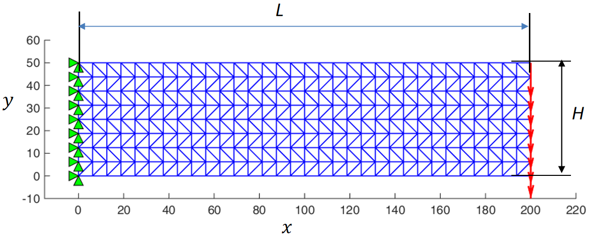
The example is a rectangular cantilever fixed at $x=0$ and loaded at $x=L$ by a total downward force distributed over the end nodes.

Length

L=200\ \mathrm{mm}

Height

H=50\ \mathrm{mm}

Thickness

h=5\ \mathrm{mm}

Young's modulus

E=2.1\times10^5\ \mathrm{MPa}

Poisson's ratio

\nu=0.3

End force

F_0=1000\ \mathrm{N}

Rectangular cantilever discretized with a CST triangular mesh — **Figure 2.** CST mesh, supports at $x=0$ , and distributed nodal forces at $x=L$ .

The mesh contains 40 subdivisions along the beam and 16 through the height: 1280 CST finite elements, 697 nodes, and 1394 equations.

gen defines the data, generates the mesh, applies the fixed-end constraints, and distributes the end force.
triang2d forms the element stiffness matrices, assembles the global system, imposes the boundary conditions, and solves for the nodal displacements.
plot_disp plots the selected displacement component.
plot_stress calculates element stresses, forms nodally averaged values, and plots the selected stress component.

Displacement and stress results

The program was executed in MATLAB R2026a. The four contour maps below use the turbo(16) colormap; the numerical calculations and plotted data are unchanged.

Horizontal displacement contour map — **Figure 3.** Horizontal displacement $u$ .

Vertical displacement contour map — **Figure 4.** Vertical displacement $v$ .

Normal stress sigma x contour map — **Figure 5.** Normal stress $\sigma_x$ .

Shear stress tau xy contour map — **Figure 6.** Shear stress $\tau_{xy}$ .

Quantity	Minimum	Maximum
$u$	$-0.0449544\ \mathrm{mm}$	$0.0449544\ \mathrm{mm}$
$v$	$-0.249364\ \mathrm{mm}$	$0\ \mathrm{mm}$
$\sigma_x$	$-93.9528\ \mathrm{MPa}$	$93.9528\ \mathrm{MPa}$
$\tau_{xy}$	$-14.2312\ \mathrm{MPa}$	$0.518913\ \mathrm{MPa}$

The calculated extrema agree with the values reported in the numerical example after rounding. The MATLAB results also agree very closely with the ANSYS comparison results.

Limitation of the CST shear-stress field

The shear stress $\tau_{xy}$ is poorly represented by the CST mesh used here. This is a consequence of the constant-stress approximation within each triangular element. In Section 9.4, the same problem will be analyzed with a four-node isoparametric quadrilateral element; for a comparable mesh density, the $\tau_{xy}$ distribution is represented much more accurately.

Programs and downloads

Verification status

The program was executed in MATLAB R2026a and reproduced all four published extrema. The ANSYS macro was inspected against the MATLAB geometry, material, thickness, mesh, constraints, and total load, but was not executed.

MCST MATLAB package5 MATLAB files and README · tested in MATLAB R2026aDownload ZIP AANSYS comparison packageMechanical APDL macro and README · inspected, not executedDownload ZIP

Reference

C. A. Felippa, Introduction to Finite Element Methods, University of Colorado Boulder, course notes and syllabus.