11. “Exact” Strains

Exact geometrical measures

Hypotheses

Large displacements and small strains.

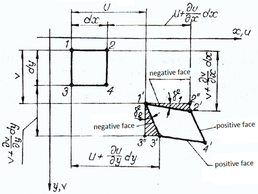
Consider the infinitesimal rectangle $1234$ in the undeformed body. The motion contains rigid-body translation and rotation together with deformation, as discussed in Chapter 10. After deformation, the rectangle becomes the parallelogram $1'2'3'4'$ .

Infinitesimal rectangle before deformation and the corresponding deformed parallelogram — **Figure 1.** Infinitesimal rectangle 1234 and its deformed configuration 1′2′3′4′.

All displacement derivatives are evaluated with respect to the coordinates of the undeformed configuration. The exact strains are:

e_x=\frac{\overline{1'2'}-\overline{12}}{\overline{12}}

e_x=\frac{\sqrt{\left(\overline{1'2''}\right)^2+\left(\overline{2'2''}\right)^2}-\overline{12}}{\overline{12}}

e_x=\frac{\sqrt{\left(dx+\dfrac{\partial u}{\partial x}\,dx\right)^2+\left(\dfrac{\partial v}{\partial x}\,dx\right)^2}-dx}{dx}

e_x=\sqrt{\left(1+\frac{\partial u}{\partial x}\right)^2+\left(\frac{\partial v}{\partial x}\right)^2}-1

Analogously, for the material fiber initially coincident with $1-3$ :

e_y=\frac{\overline{1'3'}-\overline{13}}{\overline{13}}

e_y=\frac{\sqrt{\left(\overline{1'3''}\right)^2+\left(\overline{3'3''}\right)^2}-\overline{13}}{\overline{13}}

e_y=\frac{\sqrt{\left(dy+\dfrac{\partial v}{\partial y}\,dy\right)^2+\left(\dfrac{\partial u}{\partial y}\,dy\right)^2}-dy}{dy}

e_y=\sqrt{\left(1+\frac{\partial v}{\partial y}\right)^2+\left(\frac{\partial u}{\partial y}\right)^2}-1

The decrease of the initially right angle is the sum of the rotations of the two material fibers:

\alpha_{xy}=\alpha_1+\alpha_2

\alpha_{xy}=\arctan\left(\frac{\overline{2'2''}}{\overline{1'2''}}\right)+\arctan\left(\frac{\overline{3'3''}}{\overline{1'3''}}\right)

\alpha_{xy}=\arctan\left(\frac{\dfrac{\partial v}{\partial x}\,dx}{dx+\dfrac{\partial u}{\partial x}\,dx}\right)+\arctan\left(\frac{\dfrac{\partial u}{\partial y}\,dy}{dy+\dfrac{\partial v}{\partial y}\,dy}\right)

\alpha_{xy}=\arctan\left(\frac{\partial v/\partial x}{1+\partial u/\partial x}\right)+\arctan\left(\frac{\partial u/\partial y}{1+\partial v/\partial y}\right)

Here, $e_x$ and $e_y$ denote the exact relative changes in length of the two initially orthogonal material fibers, while $\alpha_{xy}$ denotes, according to the sign convention of Figure 1, the decrease of the initial right angle between them.

A comma in the subscript denotes differentiation with respect to the coordinate that follows it. In this compact notation, the exact geometrical measures are [1]:

\left\{\begin{aligned}e_x&=\sqrt{(1+u_{,x})^2+v_{,x}^2}-1\\[4pt]e_y&=\sqrt{(1+v_{,y})^2+u_{,y}^2}-1\\[4pt]\alpha_{xy}&=\arctan\left(\frac{v_{,x}}{1+u_{,x}}\right)+\arctan\left(\frac{u_{,y}}{1+v_{,y}}\right)\end{aligned}\right.\tag{*}

The quotation marks in “Exact” Strains are intentional: these quantities have exact geometrical meanings, but, as shown below, they do not form the components of a second-order tensor.

Rigid-body rotation

As in Chapter 10, consider a rigid-body rotation through the angle $\theta$ . With:

\boldsymbol{R}=\begin{bmatrix}\cos\theta&-\sin\theta\\[3pt]\sin\theta&\cos\theta\end{bmatrix},\;\hat{\boldsymbol{x}}=\boldsymbol{R}\boldsymbol{x},\;\boldsymbol{u}=\hat{\boldsymbol{x}}-\boldsymbol{x},\;\boldsymbol{u}=\boldsymbol{R}\boldsymbol{x}-\boldsymbol{x}

\begin{aligned}\boldsymbol{R}&=\begin{bmatrix}\cos\theta&-\sin\theta\\[3pt]\sin\theta&\cos\theta\end{bmatrix},\quad \hat{\boldsymbol{x}}=\boldsymbol{R}\boldsymbol{x}\\[5pt]\boldsymbol{u}&=\hat{\boldsymbol{x}}-\boldsymbol{x},\quad \boldsymbol{u}=\boldsymbol{R}\boldsymbol{x}-\boldsymbol{x}\end{aligned}

the displacement gradients are:

\frac{\partial u}{\partial x}=\cos\theta-1,\qquad \frac{\partial u}{\partial y}=-\sin\theta

\frac{\partial v}{\partial x}=\sin\theta,\qquad \frac{\partial v}{\partial y}=\cos\theta-1

Substitution into the exact geometrical measures gives:

e_x=\sqrt{\cos^2\theta+\sin^2\theta}-1=0

e_y=\sqrt{\sin^2\theta+\cos^2\theta}-1=0

\alpha_{xy}=\arctan\!\left(\frac{-\sin\theta}{\cos\theta}\right)+\arctan\!\left(\frac{\sin\theta}{\cos\theta}\right)=0

Rigid-body check

e_x=0,\qquad e_y=0,\qquad \alpha_{xy}=0

Thus, like the Green–Lagrange strain discussed in Chapter 10, these geometrical measures correctly filter out rigid-body translation and rotation.

Linearized strain tensor

The familiar linearized strain components are:

\varepsilon_x=u_{,x},\qquad \varepsilon_y=v_{,y},\qquad \gamma_{xy}=u_{,y}+v_{,x}

They form the symmetric second-order tensor:

\boldsymbol{\varepsilon}=\begin{bmatrix}\varepsilon_x&\gamma_{xy}/2\\[5pt]\gamma_{xy}/2&\varepsilon_y\end{bmatrix}

The quantities $\varepsilon_x$ , $\varepsilon_y$ , and $\gamma_{xy}/2$ are components of the tensor; $\gamma_{xy}$ is the shear strain in the usual engineering notation.

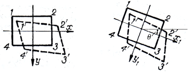
Strain components represented in an initial and a rotated coordinate frame — **Figure 2.** Strain components in the original and rotated coordinate frames.

If the reference frame is rotated through the angle $\theta$ , with:

\mathbf R=\begin{bmatrix}\cos\theta&\sin\theta\\[3pt]-\sin\theta&\cos\theta\end{bmatrix}

the tensor components in the rotated frame are:

\boldsymbol{\varepsilon}_1=\mathbf R\boldsymbol{\varepsilon}\mathbf R^{T}

The numerical components change with the reference frame, but the physical tensor is unchanged; its components obey the tensor transformation law [2].

Green–Lagrange strain tensor

Green–Lagrange strain is also a symmetric second-order tensor:

\mathbf E_1=\mathbf R\mathbf E\mathbf R^{T}

In compact form:

\boxed{\mathbf E=\frac12\left[\nabla\mathbf u+(\nabla\mathbf u)^{T}\right]+\frac12(\nabla\mathbf u)^{T}\nabla\mathbf u}

where:

\nabla\mathbf u=\begin{bmatrix}u_{,x}&u_{,y}\\[5pt]v_{,x}&v_{,y}\end{bmatrix}

The first term is the linearized strain tensor, while the second term contains the quadratic contributions responsible for the geometrically nonlinear strain–displacement relation.

Fundamental distinction

The geometrical quantities $e_x$ , $e_y$ , and $\alpha_{xy}$ have exact geometrical meanings, but they do not constitute the components of a second-order tensor. This distinguishes them fundamentally from both the linearized strain tensor and the Green–Lagrange strain tensor.

Exact relations and small-strain limit

For the material fiber initially parallel to $x$ , the stretch is $\lambda_x=1+e_x$ . Therefore:

E_{xx}=\frac12(\lambda_x^2-1)=\frac12\left[(1+e_x)^2-1\right]=e_x+\frac12e_x^2

Analogously, $\lambda_y=1+e_y$ . Hence:

\boxed{E_{xx}=e_x+\frac12e_x^2}

\boxed{E_{yy}=e_y+\frac12e_y^2}

\boxed{2E_{xy}=(1+e_x)(1+e_y)\sin\alpha_{xy}}

A short geometrical derivation of these exact relations can be found here.

The shear relation follows from the exact angle between the two deformed material fibers: their stretches are $1+e_x$ and $1+e_y$ , while the cosine of their deformed included angle is $\cos(\pi/2-\alpha_{xy})=\sin\alpha_{xy}$ . It is therefore not a direct axial analogue; it is the exact relation between the Green–Lagrange shear component and the geometrical changes in length and angle.

These relations are exact, not approximations.

For:

|e_x|\ll1,\qquad |e_y|\ll1,\qquad |\alpha_{xy}|\ll1

the exact relations reduce to:

E_{xx}\approx e_x,\qquad E_{yy}\approx e_y,\qquad 2E_{xy}\approx\alpha_{xy}

Only when displacements and rotations are also small do the familiar linearized strain expressions follow:

\varepsilon_x=u_{,x},\qquad \varepsilon_y=v_{,y},\qquad \gamma_{xy}=u_{,y}+v_{,x}

Small strains alone do not justify the linearized kinematics, because small strains may coexist with large rotations.

Connection to Chapter 12

The important point for the following chapters is that Green–Lagrange strains remain suitable when displacements and rotations are large while the actual strains remain small. This is precisely the situation considered in the Total Lagrangian formulation presented in the next chapter.

References

Deformation (physics). Wikipedia.
Allan F. Bower, A Brief Introduction to Tensors and Their Properties, Appendix B of Applied Mechanics of Solids. Applied Mechanics of Solids.