Section 12.1 of Chapter 12: Total Lagrangian Formulation (TL)
CST Finite Element
A complete Total Lagrangian formulation of the plane-stress constant-strain triangle for small strains and large displacements, including the consistent tangent stiffness matrix and two verified nonlinear examples.
Total LagrangianPlane stressCSTMATLABANSYS
01
Formulation and hypotheses
StrainSmall
DisplacementLarge
MaterialLinear elastic
Stress statePlane stress
In the Total Lagrangian formulation, the initial undeformed geometry is the reference configuration. All derivatives and integrals are evaluated with respect to that initial configuration, and the Green–Lagrange strain measure is used.
Because the strains and stresses are constant within each plane-stress CST finite element, the deformation energy is:
U=21Ael=1nel(∫AelhεTσdA)
U=21Ael=1nel(εTσVel)
Here, Ael=1nel denotes the standard finite element assembly operation from the first through the last element. The signed element area is:
Ael=21[(x2−x1)(y3−y1)−(x3−x1)(y2−y1)]
The sign of Ael depends on whether the element nodes are numbered counterclockwise or clockwise. The physical area is ∣Ael∣, and the element volume is:
Vel=h∣Ael∣
h is the element thickness, and nel is the number of finite elements.
02
Strain and stress measures
ε=⎩⎨⎧εxεyγxy⎭⎬⎫
σ=⎩⎨⎧σxσyτxy⎭⎬⎫
The engineering shear component satisfies γxy=2Exy. For a linear elastic material in plane stress:
σ=Dε
D=1−ν2E1ν0ν100021−ν
The two-dimensional Green–Lagrange strain components are:
εx=∂x∂u+21(∂x∂u)2+21(∂x∂v)2
εy=∂y∂v+21(∂y∂u)2+21(∂y∂v)2
γxy=∂y∂u+∂x∂v+∂x∂u∂y∂u+∂x∂v∂y∂v
03
CST interpolation
The displacement field is interpolated with the same linear functions used in the CST element of Section 9.1:
Here, V=−uTF is the potential of the external loads, u is the global nodal displacement vector, and F is the global external force vector. The virtual-work equation is:
δΠ=Ael=1nel(δεTσVel)−δuTF=0
δΠ=Ael=1nel(δuelTBTσVel)−δuTF=0
This relation holds for every geometrically admissible virtual displacement field. The resulting nonlinear equilibrium system is:
Ψ(u)=Ael=1nel(BTσVel)−F=0
Ψ(u)=Ael=1nel[(B0T+BLT(uel))σVel]−F=0
07
Tangent stiffness matrix
The first variation of the equilibrium residual is:
The tangent stiffness matrix of one CST finite element is:
kel=Vel(σxGx+σyGy+τxyGxy+BTDB)
The first term is the geometric or stress-dependent part; the second is the material part. Equivalently:
Ψ(u)=Ael=1nelfel−F=0,fel=BTσVel
kel=∂uel∂fel,KT=Ael=1nelkel=∂u∂Ψ
08
Newton–Raphson solution
At Newton–Raphson iteration i:
Δu(i)=−(KT(i))−1Ψ(i)
u(i+1)=u(i)+Δu(i)
Ψ(i)=Ψ(u(i))
The element internal-force vectors and tangent stiffness matrices are assembled in the standard way. A convenient stopping measure is:
ϵ=nΔuTΔu
where n is the total number of equations.
Important remark #1
The Total Lagrangian formulation presented here is not based on an incremental strain approximation. The equilibrium equations are written directly with respect to the initial configuration. Therefore, the accuracy of the formulation itself does not depend on the number of load steps. For problems with moderate nonlinearity, a single load step may be sufficient, provided that the Newton–Raphson iterations converge. Additional load steps may nevertheless be useful to improve convergence in more strongly nonlinear problems.
09
Example 1. Pure Bending of a Cantilever Beam
The cantilever has length L=400mm, a rectangular cross-section with thickness 5mm and height 20mm, E=1000MPa, and ν=0.3. It is subjected to the end moment M=19000Nmm. The mesh has 60 subdivisions along the beam and 16 through its height: 1,920 CST elements and 1,037 nodes.
The analytical total rotation is:
θ=EIML=1000⋅5⋅1220319000⋅400=2.267rad=129.9∘
This analytical value is practically identical to that obtained with the finite-element model.
Figure 1. Deformed configuration and normal stress σx under pure bending.Figure 2. Green–Lagrange axial strain εx.
10
Example 2. Cantilever Beam Subjected to a Tip Force
The same beam geometry and material are used, with a vertical force F=100N applied at the free end. The mesh has 120 subdivisions along the beam and 16 through its height: 3,840 CST elements and 2,057 nodes.
ANSYS uses an Updated Lagrangian formulation for this large-displacement analysis and reports Cauchy stresses and logarithmic strains in the rotated element coordinate system. Since the strains in the present example remain small, these results can be meaningfully compared with the Green–Lagrange strains and second Piola–Kirchhoff stresses obtained with the present Total Lagrangian formulation.
The displacement results are:
Figure 3. Vertical displacement v.Figure 4. Horizontal displacement u.
∣vmax∣MATLAB=286.4mm,∣umax∣MATLAB=156.3mm
∣vmax∣ANSYS=287.1mm,∣umax∣ANSYS=156.8mm
The normal-stress and Von Mises stress results are:
Figure 5. Second Piola–Kirchhoff normal stress σx.Figure 6. Von Mises stress σVM.
σx,minMATLAB=−78.9MPa,σx,maxMATLAB=80.2MPa
σx,minANSYS=−80.4MPa,σx,maxANSYS=78.7MPa
σVM,maxMATLAB=74.9MPa,σVM,maxANSYS=74.1MPa
Figure 7. Green–Lagrange axial strain εx.
εx,minMATLAB=−0.0718,εx,maxMATLAB=0.0729
εx,minANSYS=−0.0732,εx,maxANSYS=0.0716
The agreement between the MATLAB and ANSYS results is very good for displacements, stresses, and strains.
Important remark #2
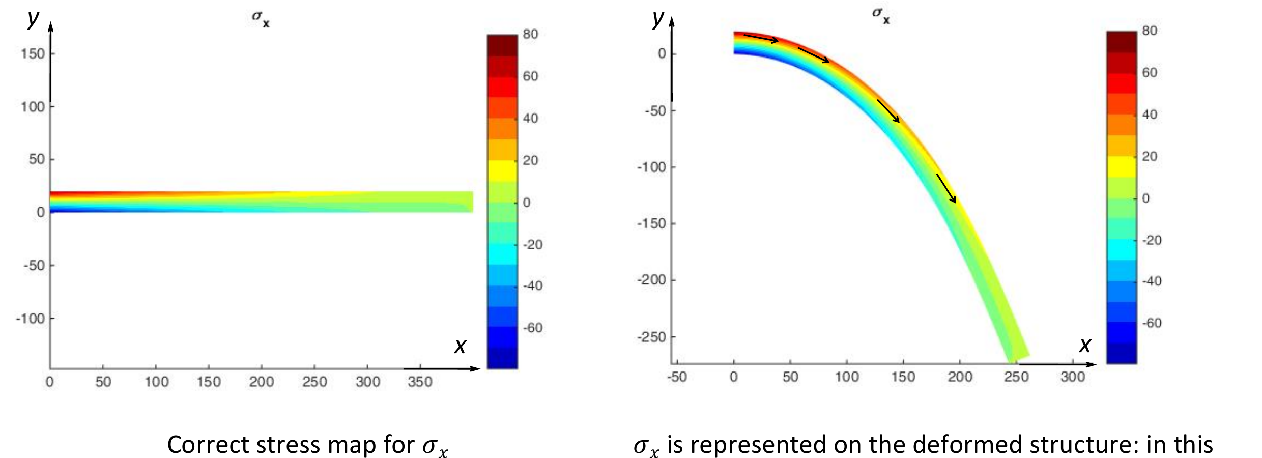
In the Total Lagrangian formulation, strains and stresses are referred to the initial undeformed configuration. Therefore, the mathematically consistent stress map is the one represented on the initial geometry, as shown on the left.
For a more intuitive visualization, the same second Piola–Kirchhoff stresses may also be represented on the deformed geometry, as shown on the right. In this representation, the material directions rotate together with the finite elements; therefore, the x-stress direction becomes approximately tangent to the deformed beam axis.
Cauchy stresses are defined in the current configuration. When strains are small, their values referred to the corresponding local, rotated material directions are very close to the second Piola–Kirchhoff stresses. The distinction becomes important when comparing stress components expressed in different reference frames.
Figure 8. The stress direction is fixed with respect to the initial reference frame on the left and rotates with the material directions in the deformed visualization on the right. The explanatory arrows are retained from the author's figure.
The MATLAB package was executed in MATLAB R2026a. All five load steps reached convergence, and the numerical values reproduced the documented results. The ANSYS macro was inspected for consistency with the geometry, thickness, material, plane-stress assumption, loading, constraints, and mesh of Example 2, but it was not executed.