10. Green–Lagrange Strain Tensor

Large motion and linearized strain

Hypothesis

Large displacements and small strains.

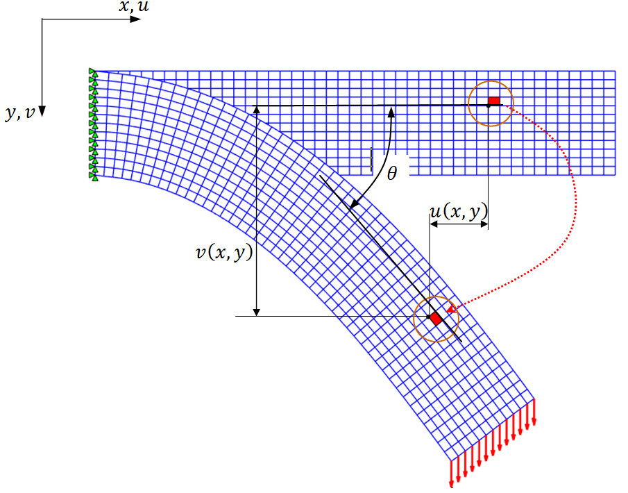
A body may undergo large displacements while its local dimensions change only slightly. The important difficulty arises mainly from large rigid-body rotations: a constant rigid translation produces no displacement gradients, whereas a finite rotation produces gradients that the linearized strain tensor does not remove.

Conceptually, the motion may be regarded locally as a rigid-body translation and rotation combined with a small deformation. This decomposition is useful for interpretation, but it is local and is not unique.

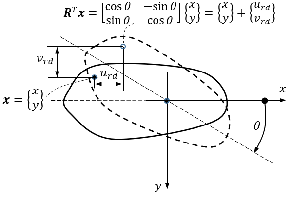
Finite element mesh undergoing a large rotation and a small local deformation — **Figure 1.** Left: large motion with small local deformation. Right: finite rigid-body rotation and its displacement field.

Rigid-body rotation and the corresponding displacement components — **Figure 1.** Left: large motion with small local deformation. Right: finite rigid-body rotation and its displacement field.

The usual engineering strains — more precisely, the components of the linearized strain tensor — are adequate for small-displacement problems. This is the strain measure usually introduced first in undergraduate engineering courses.

Consider a rigid rotation through the angle $\theta$ about the origin:

\widehat{\boldsymbol{x}}=\boldsymbol{R}\boldsymbol{x},\qquad \boldsymbol{u}_{rd}=\widehat{\boldsymbol{x}}-\boldsymbol{x}=(\boldsymbol{R}-\boldsymbol{I}_2)\boldsymbol{x}

\boldsymbol{x}=\begin{Bmatrix}x\\[3pt]y\end{Bmatrix},\qquad \boldsymbol{R}=\begin{bmatrix}\cos\theta&-\sin\theta\\[3pt]\sin\theta&\cos\theta\end{bmatrix}

The components of the rigid-rotation displacement field are:

u_{rd}=(\cos\theta-1)x-\sin\theta\,y,\qquad v_{rd}=\sin\theta\,x+(\cos\theta-1)y

Substitution into the linearized strain components gives:

\varepsilon_x^{\mathrm{lin}}=\frac{\partial u_{rd}}{\partial x}=\cos\theta-1,\qquad \varepsilon_y^{\mathrm{lin}}=\frac{\partial v_{rd}}{\partial y}=\cos\theta-1

\gamma_{xy}^{\mathrm{lin}}=\frac{\partial u_{rd}}{\partial y}+\frac{\partial v_{rd}}{\partial x}=-\sin\theta+\sin\theta=0

Thus, although the body has not deformed, a plane-stress Hooke law would produce the spurious stresses:

\begin{Bmatrix}\sigma_x\\[3pt]\sigma_y\\[3pt]\tau_{xy}\end{Bmatrix}=\frac{E}{1-\nu^2}\begin{bmatrix}1&\nu&0\\[3pt]\nu&1&0\\[3pt]0&0&\dfrac{1-\nu}{2}\end{bmatrix}\begin{Bmatrix}\cos\theta-1\\[3pt]\cos\theta-1\\[3pt]0\end{Bmatrix}

\sigma_x=\sigma_y=\frac{E}{1-\nu}(\cos\theta-1),\qquad \tau_{xy}=0

Finite-strain measures therefore have to predict zero strain for arbitrary rigid-body motion and reduce to the linearized strain tensor when their nonlinear terms are neglected [1].

Green–Lagrange strain tensor

Let the initial and deformed coordinates of a material point be:

\boldsymbol{x}=\begin{Bmatrix}x\\[3pt]y\end{Bmatrix},\qquad \widehat{\boldsymbol{x}}=\begin{Bmatrix}\hat{x}\\[3pt]\hat{y}\end{Bmatrix}=\boldsymbol{x}+\boldsymbol{u},\qquad \boldsymbol{u}=\begin{Bmatrix}u\\[3pt]v\end{Bmatrix}

All displacement derivatives in this chapter are calculated with respect to the coordinates $x,y$ of the initial, undeformed configuration. The displacement gradient is denoted by:

\nabla\boldsymbol{u}=\begin{bmatrix}\dfrac{\partial u}{\partial x}&\dfrac{\partial u}{\partial y}\\[6pt]\dfrac{\partial v}{\partial x}&\dfrac{\partial v}{\partial y}\end{bmatrix}

The deformation gradient is therefore:

\boldsymbol{F}=\frac{\partial\widehat{\boldsymbol{x}}}{\partial\boldsymbol{x}}=\boldsymbol{I}_2+\nabla\boldsymbol{u}

\boldsymbol{F}=\begin{bmatrix}\dfrac{\partial\hat{x}}{\partial x}&\dfrac{\partial\hat{x}}{\partial y}\\[7pt]\dfrac{\partial\hat{y}}{\partial x}&\dfrac{\partial\hat{y}}{\partial y}\end{bmatrix}=\boldsymbol{I}_2+\begin{bmatrix}\dfrac{\partial u}{\partial x}&\dfrac{\partial u}{\partial y}\\[7pt]\dfrac{\partial v}{\partial x}&\dfrac{\partial v}{\partial y}\end{bmatrix}

d\widehat{\boldsymbol{x}}=\boldsymbol{F}\,d\boldsymbol{x}

The change in the squared length of the differential vector is:

d\widehat{\boldsymbol{x}}^{T}d\widehat{\boldsymbol{x}}-d\boldsymbol{x}^{T}d\boldsymbol{x}=d\boldsymbol{x}^{T}\boldsymbol{F}^{T}\boldsymbol{F}\,d\boldsymbol{x}-d\boldsymbol{x}^{T}d\boldsymbol{x}

=d\boldsymbol{x}^{T}(\boldsymbol{F}^{T}\boldsymbol{F}-\boldsymbol{I}_2)d\boldsymbol{x}=2d\boldsymbol{x}^{T}\boldsymbol{E}\,d\boldsymbol{x}

Hence, the Green–Lagrange strain tensor is:

\boldsymbol{E}=\frac12\left(\boldsymbol{F}^{T}\boldsymbol{F}-\boldsymbol{I}_2\right)

Or, using the displacement gradient:

\boldsymbol{E}=\frac12\left[\nabla\boldsymbol{u}+\left(\nabla\boldsymbol{u}\right)^{T}+\left(\nabla\boldsymbol{u}\right)^{T}\nabla\boldsymbol{u}\right]

Or:

\left\{\begin{aligned} E_x={}&\frac{\partial u}{\partial x}+\frac12\left(\frac{\partial u}{\partial x}\right)^2+\frac12\left(\frac{\partial v}{\partial x}\right)^2\\[7pt] E_y={}&\frac{\partial v}{\partial y}+\frac12\left(\frac{\partial u}{\partial y}\right)^2+\frac12\left(\frac{\partial v}{\partial y}\right)^2\\[7pt] E_{xy}={}&\frac12\left(\frac{\partial u}{\partial y}+\frac{\partial v}{\partial x}\right)\\[3pt] &+\frac12\left(\frac{\partial u}{\partial x}\frac{\partial u}{\partial y}+\frac{\partial v}{\partial x}\frac{\partial v}{\partial y}\right) \end{aligned}\right.

Green–Lagrange strains with engineering notations $(\gamma_{xy}=2E_{xy})$ :

\left\{\begin{aligned} \varepsilon_x={}&\frac{\partial u}{\partial x}+\frac12\left(\frac{\partial u}{\partial x}\right)^2+\frac12\left(\frac{\partial v}{\partial x}\right)^2\\[7pt] \varepsilon_y={}&\frac{\partial v}{\partial y}+\frac12\left(\frac{\partial u}{\partial y}\right)^2+\frac12\left(\frac{\partial v}{\partial y}\right)^2\\[7pt] \gamma_{xy}={}&\frac{\partial u}{\partial y}+\frac{\partial v}{\partial x}\\[3pt] &+\frac{\partial u}{\partial x}\frac{\partial u}{\partial y}+\frac{\partial v}{\partial x}\frac{\partial v}{\partial y} \end{aligned}\right.

Using comma notation, in which a comma in the subscript denotes partial differentiation with respect to the following coordinate—for example, $u_{,x}\equiv\partial u/\partial x$ —the Green–Lagrange strains may also be written as:

\left\{\begin{aligned} \varepsilon_x={}&u_{,x}+\frac12u_{,x}^{2}+\frac12v_{,x}^{2}\\[7pt] \varepsilon_y={}&v_{,y}+\frac12u_{,y}^{2}+\frac12v_{,y}^{2}\\[7pt] \gamma_{xy}={}&u_{,y}+v_{,x}+u_{,x}u_{,y}+v_{,x}v_{,y} \end{aligned}\right.

Rigid-body motion

For a rigid-body translation and rotation:

\widehat{\boldsymbol{x}}=\boldsymbol{R}\boldsymbol{x}+\boldsymbol{c}

where the constant translation $\boldsymbol{c}$ has zero gradient. Therefore, for the rotation:

u_{rd,x}=\cos\theta-1,\qquad u_{rd,y}=-\sin\theta,\qquad v_{rd,x}=\sin\theta,\qquad v_{rd,y}=\cos\theta-1

\boldsymbol{F}=\frac{\partial\widehat{\boldsymbol{x}}}{\partial\boldsymbol{x}}=\boldsymbol{R}

\boldsymbol{E}=\frac12\left(\boldsymbol{R}^{T}\boldsymbol{R}-\boldsymbol{I}_2\right)=\boldsymbol{0}

Rigid-body translation and rotation do not produce Green–Lagrange strain. In this sense, Green–Lagrange strain “filters out” rigid-body motion [1].

One-dimensional comparison

Consider a prismatic bar fixed at one end and subjected to axial tension. Its initial length is $L_0$ , its final length is $L=L_0+u$ , and $u$ is the displacement of the free end.

The engineering axial strain is:

e=\frac{L-L_0}{L_0}=\frac{u}{L_0}

The one-dimensional Green–Lagrange strain is:

E=\frac{L^2-L_0^2}{2L_0^2}=\frac{(L_0+u)^2-L_0^2}{2L_0^2}=\frac{u}{L_0}+\frac{u^2}{2L_0^2}

Direct relation

E=e+\frac12e^2

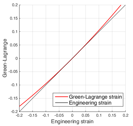
Comparison between one-dimensional Green-Lagrange strain and engineering axial strain — **Figure 2.** Green–Lagrange strain compared with engineering axial strain.

For axial tension, the relative difference follows immediately:

\frac{E-e}{e}=\frac{e}{2}

Thus, for $e=5\%$ , the relative difference is $2.5\%$ ; for $e=10\%$ , it is $5\%$ . In ordinary elastic applications, the axial strain of steel is generally much smaller than $1\%$ .

e\ll1\qquad\Longrightarrow\qquad E\approx e

Small-strain limit and stresses

When the displacement-gradient quadratic terms are negligible, the Green–Lagrange components reduce to the components of the linearized strain tensor:

\varepsilon_x\approx u_{,x},\qquad \varepsilon_y\approx v_{,y},\qquad \gamma_{xy}\approx u_{,y}+v_{,x}

When both strains and displacements are small, the Green–Lagrange strains are very close to the usual linearized strains. Therefore, for a linear elastic material, the stresses can be obtained using the usual Hooke law:

\boldsymbol{\sigma}=\boldsymbol{D}\boldsymbol{\varepsilon}

\begin{Bmatrix}\sigma_x\\[3pt]\sigma_y\\[3pt]\tau_{xy}\end{Bmatrix}=\frac{E}{1-\nu^2}\begin{bmatrix}1&\nu&0\\[3pt]\nu&1&0\\[3pt]0&0&\dfrac{1-\nu}{2}\end{bmatrix}\begin{Bmatrix}\varepsilon_x\\[3pt]\varepsilon_y\\[3pt]\gamma_{xy}\end{Bmatrix}

Here $E$ is Young's modulus and $\nu$ is Poisson's ratio.

In a fully finite-deformation formulation, Green–Lagrange strain is naturally associated with the second Piola–Kirchhoff stress measure, but this distinction is not needed here. In the following chapters, the main advantage of Green–Lagrange strain will be used directly: it allows large displacements and rotations while the strains remain small.

Reference

Nam-Ho Kim, Introduction to Nonlinear Finite Element Analysis, Springer, 2015. Springer.