01
Formulation and tangent stiffness
Although the displacements are assumed to be small, the second-order terms in the strain–displacement relations are retained because they are essential for the stability analysis. These terms generate the geometric stiffness matrix.
Buckling is a bifurcation phenomenon. The structure follows the small-displacement equilibrium path up to a critical load, at which this equilibrium state loses stability and a new equilibrium path associated with lateral deformation becomes possible. Along the post-buckling path, large displacements may subsequently develop.
We will consider the quadrilateral isoparametric element with four nodes. We start from the Total Lagrangian formulation developed in Section 12.2.
For the present buckling analysis, the small-displacement assumption is adopted, but the second-order strain terms responsible for the geometric stiffness are retained. The overall tangent stiffness matrix has the form:
For all notations, see Section 12.2. Starting from the tangent stiffness matrix of the TL formulation, the displacement-dependent part associated with the large-displacement contribution to the strain–displacement matrix is neglected under the small-displacement assumption. The stress-dependent terms are retained because they form the geometric stiffness matrix and are essential for the stability analysis. Therefore:
The elastic stiffness matrix and the geometric stiffness matrix , which depends on the stress state, are:
The sign convention is:
Consequently, the minus sign in the definition above makes positive in the destabilizing direction for a compressive reference stress state. After assembly and application of the boundary conditions, the buckling problem is:
or, equivalently:
02
Element matrices
To find the matrices and for one finite element, the same procedure as in Chapter 19 is used. The 2D Green–Lagrange strains, including the second-order terms, are:
Equivalently, the strain vector is separated into its linear and second-order parts:
The first derivatives of the displacements are obtained from the shape functions as in Section 12.2:
Thus:
Then the deformation energy for one finite element is calculated:
Here is the element area in the plane, and is the constant thickness used in the program.
After substitution of the strain expression in the strain energy and neglecting terms of order higher than two, the expression can be separated into an elastic part and a part that depends on the stresses. The matrix is substituted with . The two element matrices are:
The matrices and for all finite elements are assembled in the standard way to obtain the global matrices and , after which the boundary conditions are applied.
03
MATLAB programs
To solve the eigenvalue problem, that is, to compute numerically the eigenvalues and eigenvectors, the MATLAB command eig or eigs can be used. Usually, only the smallest critical eigenvalue is of interest. The eigs command is preferable for sparse matrices.
Prior to solving the eigenvalue problem, the linear static problem must be solved to determine the stress state in the finite elements. The main program is:
% *** main ***
clear
gen
stiff
S=K\F;
stress
geomK
The gen subprogram generates the input data. The stiff subprogram generates the elastic stiffness matrix and applies the boundary conditions, using the Q4 formulation developed in Section 9.4. The linear system is then solved. The stress subprogram computes the stresses in all finite elements, and geomK generates the geometric stiffness matrix and solves the eigenvalue problem.
In the distributed program, the robust sparse reciprocal eigenproblem is solved and the required load multipliers are obtained from . This is algebraically equivalent to .
04
Example 1
A 0.5 m long cantilever beam with a square cross-section having a side of is compressed by a force of . Young's modulus is , and Poisson's ratio is .
The Euler buckling load is [1]:
The result depends on the mesh, as shown in the table below.
| Mesh (height × length) | MATLAB (N) | ANSYS (N) |
|---|---|---|
| 6 × 50 | 30331.6 | 30352.3 |
| 8 × 100 | 28305.6 | 28324.5 |
| 10 × 200 | 27792.0 | 27810.4 |
| 12 × 250 | 27723.9 | 27742.2 |
| 6 × 250 | 27781.1 | — |
| 15 × 300 | 27684.5 | 27702.7 |
| 6 × 300 | 27748.6 | — |
The relatively slow convergence is mainly due to the use of bilinear Q4 plane-stress elements for a slender, bending-dominated member. Unlike beam elements, Q4 elements do not reproduce the bending field exactly and therefore require a relatively fine mesh. The additional results obtained with and elements show that, for this example, refinement along the beam length is particularly effective: even with only six elements through the height, the critical load approaches the converged value closely. This also explains why the beam elements used in Chapter 19 converge much faster for the same physical phenomenon: beam elements are specifically formulated to represent bending behaviour efficiently, whereas the Q4 plane-stress element must reproduce the same bending field through mesh refinement.
05
Q8 finite element
The same buckling problem was also solved using the isoparametric Q8 element. The buckling procedure remains unchanged; only the interpolation changes from Q4 to Q8. The linear Q8 element is presented in Section 9.6, and its Total Lagrangian formulation in Section 12.3.
| Mesh (height × length) | Critical load [N] |
|---|---|
| 1 × 8 | 27851.247 |
| 2 × 16 | 27680.620 |
| 3 × 25 | 27654.802 |
| 4 × 32 | 27647.495 |
| 6 × 40 | 27642.983 |
| 8 × 100 | 27636.673 |
| Euler beam solution | 27635 |
Q8 gives very good results even for relatively coarse meshes. For the 1 × 8 mesh, the difference from the Euler beam solution is approximately 0.78%; for 3 × 25, it is already below 0.1%. Q8 converges much faster than Q4 in this bending-dominated problem. The slow convergence observed previously with Q4 is therefore mainly associated with the Q4 interpolation, not with the buckling formulation.
The MATLAB program used for the Q8 buckling analysis can be downloaded below.
06
Example 2
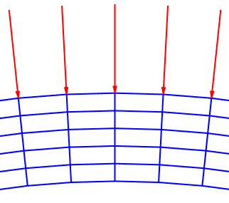
A ring is loaded as shown in Figure 2. The distributed force is equal to . The ring is free; no boundary conditions are applied. Consequently, the buckling modes are not uniquely oriented in space. If an eigenmode is rotated rigidly around the centre of the ring, the rotated shape is also an eigenmode associated with the same eigenvalue. This rotational indeterminacy explains why the eigenmodes appear in pairs with identical or nearly identical eigenvalues.
The orientation of each mode in a degenerate pair is therefore arbitrary and depends on the numerical eigensolver.
The inner diameter is ; the width and thickness are both . Young's modulus is , and Poisson's ratio is . The mesh has 10 finite elements through the width and 120 along the circumference, giving 1320 nodes and 1200 quadrilateral Q4 finite elements.
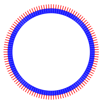
The first six eigenvectors and eigenvalues are:
07
Reference
[1] Timoshenko, S.P., Gere, J.M., Theory of Elastic Stability, McGraw-Hill, 1985.