01
Purpose and benchmark model
plane2d8_fast is the vectorized alternative to the standard plane2d8 routine presented in Section 9.6. It follows the same general strategy as the Q4 fast solver in Section 9.5: simultaneous element computations with multiprod and direct sparse assembly with MATLAB sparse.
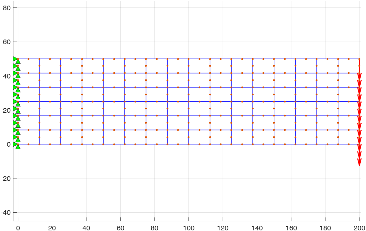
The benchmark uses the plane-stress cantilever of Section 9.6. The mesh has Q8 elements through the height and elements along the length, so that:
Each element has eight nodes and two displacement degrees of freedom per node: 16 element displacement degrees of freedom. The strain–displacement matrix is and the element stiffness matrix is . The Q8 interpolation and plane-stress formulation remain those of Section 9.6; the present section concerns their computational implementation.
02
Nine Gauss-point contributions
Each Q8 finite element is integrated with a Gauss rule, giving nine Gauss points. The number of vectorized integration contributions is therefore:
The strain–displacement and constitutive matrices are stored for every Gauss-point contribution in three-dimensional arrays:
Thus, the nine terms belonging to each finite element are evaluated vectorially. The integration factor is included in the stored constitutive array. During sparse assembly, their entries have the same element connectivity and are naturally summed at the corresponding global matrix positions.
03
Vectorized element computation
The nodal coordinate arrays are first repeated for the nine Gauss points of every element. The Q8 shape-function derivatives in natural coordinates are evaluated for all these points and stored in dNst, with dimensions . The coordinate array xyel has dimensions .
The Jacobian matrices, their inverses, and the derivatives with respect to the Cartesian coordinates are then evaluated simultaneously for all contributions:
J=multiprod(dNst,xyel);Each inverse Jacobian is formed from its determinant and four entries. The Cartesian derivatives are then obtained page-wise:
br=multiprod(J1,dNst);The Q8 strain–displacement matrix has sixteen columns. Its implementation therefore uses the explicit preallocation:
B=zeros(3,16,nel9);The constitutive matrices include the Gauss weight, the absolute Jacobian determinant, and the element thickness. The simultaneous matrix products are:
DB=multiprod(DHooke,B);
kelt=reshape(multiprod(permute(B,[2 1 3]),DB),ngel^2,nel9);
Here DB stores the products for all Gauss points, while each column of kelt contains the 256 entries of one Gauss-point stiffness contribution. multiprod performs a matrix product on each page of the arrays: page of one array is multiplied by the corresponding page of the other array. These are matrix products for all Gauss points of all elements, not element-by-element scalar products.
04
Sparse global assembly
The connectivity arrays are expanded to the nine Gauss-point contributions. MATLAB sparse then assembles the global stiffness matrix directly and sums coincident entries:
K=sparse(ipos1,ipos2(:),kelt(:),neq,neq);This avoids the element-by-element stiffness-assembly loop. Both the nine contributions of each element and the contributions of adjacent elements are added at their common global positions. After applying the constraints and loads, the global linear system is solved in the standard form:
S=K\F;The MATLAB variable S contains the global nodal displacement vector . After the solution, DHooke is restored to the unweighted plane-stress constitutive matrix used by the stress-plotting routine.
05
Use with Section 9.6
Start from the complete MATLAB programs provided in Section 9.6, add plane2d8_fast.m and multiprod.m, and replace the call plane2d8 in main.m with plane2d8_fast. The geometry, material, loading, constraints, and result-plotting routines remain unchanged.
clear
gen
plane2d8_fast
plot_disp
plot_stress
06
MATLAB R2026a benchmark
For each of the two meshes, both routines received one unrecorded warm-up run followed by three measured runs. The table reports arithmetic means measured in MATLAB 26.1.0 (R2026a) Update 4 on the same computer. Only the meshes 60 × 150 and 80 × 200 were used.
The assembly interval includes element-matrix generation, loads, constraints, and global stiffness assembly. The linear solution was measured separately. Total time is the sum of these two directly measured intervals; mesh generation and plotting are excluded.
| Elements | Nodes | Equations | Standard assembly (s) | Standard solve (s) | Standard total (s) | Fast assembly (s) | Fast solve (s) | Fast total (s) | Overall speed-up | |
|---|---|---|---|---|---|---|---|---|---|---|
| 60 × 150 | 9,000 | 27,421 | 54,842 | 31.134 | 0.420 | 31.554 | 0.620 | 0.413 | 1.033 | 30.5× |
| 80 × 200 | 16,000 | 48,561 | 97,122 | 104.531 | 0.985 | 105.516 | 1.366 | 1.119 | 2.485 | 42.5× |
The vectorized Gauss-point calculations and direct sparse assembly substantially reduce the assembly interval. The overall acceleration is smaller because the sparse linear-system solution remains essentially the same operation in both implementations.
Both meshes were also checked against the standard Q8 solution. For 60 × 150 and 80 × 200, respectively, is 3.400e-9 mm and 1.541e-8 mm; the relative differences are 1.626e-10 and 5.542e-10. The largest differences between the nodally recovered stress components and von Mises stresses are 3.213e-8 MPa and 1.224e-7 MPa. These differences are consistent with floating-point round-off from the different operation ordering.
The distinction is important: improves the finite-element approximation, particularly for bending, whereas improves the computational implementation without changing the FEM formulation. The two Q8 programs solve the same problem and must produce the same solution.
07
Programs and downloads
The standard and fast Q8 solvers were executed in MATLAB R2026a on both published benchmark meshes. The package contains the complete fast-solver example, the standard solver for comparison, multiprod, its BSD license, and a README.
multiprod.m is by Paolo de Leva and is redistributed under the included BSD-style license. Its distribution page is the MATLAB Central File Exchange entry.