Section 25.3 of Chapter 25: Hexahedral isoparametric finite element. Linear case

Hexahedral 20-node isoparametric finite element for linear analysis

01

Element and hypotheses

StrainSmall
DisplacementSmall
MaterialLinear elastic

The formulation closely follows Section 25.1. Only the differences associated with the quadratic 20-node interpolation and the 3×3×33\times3\times3 Gauss integration are presented here.

The HEX20 element has 20 nodes, three displacement DOFs per node and 60 element displacement DOFs. The stiffness integration uses 27 Gauss points.

uel∈R60×1,kel∈R60×60.\htmlClass{fea-math-bold-italic}{\boldsymbol{u}}_{el}\in\mathbb R^{60\times1},\qquad\htmlClass{fea-math-bold-italic}{\boldsymbol{k}}_{el}\in\mathbb R^{60\times60}.

02

Natural coordinates and interpolation

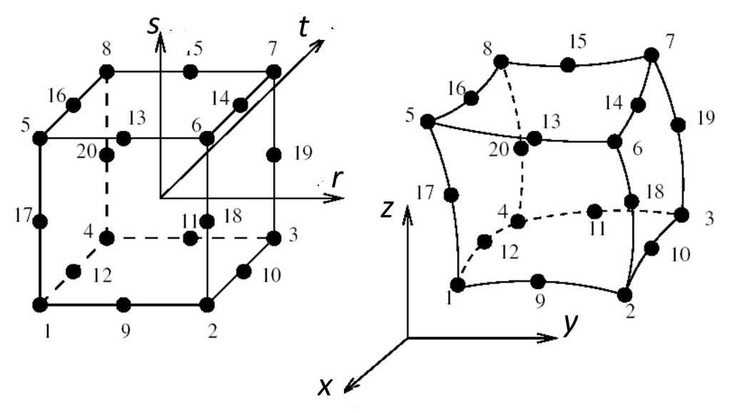
HEX20 natural coordinates s, t, r and nodal numbering; global geometry
Figure 1. Natural coordinates and nodal numbering of the HEX20 element (left), and the corresponding geometry in the global reference frame (right). Adapted from Itasca Software [1].
Natural coordinates of the HEX20 nodes.
Nodesis_itit_irir_iNodesis_itit_irir_i
1−1-1−1-1−1-111−1-1−1\phantom{-}1−0\phantom{-}0
2−1-1−1-1−1\phantom{-}112−1-1−0\phantom{-}0−1-1
3−1-1−1\phantom{-}1−1\phantom{-}113−1\phantom{-}1−1-1−0\phantom{-}0
4−1-1−1\phantom{-}1−1-114−1\phantom{-}1−0\phantom{-}0−1\phantom{-}1
5−1\phantom{-}1−1-1−1-115−1\phantom{-}1−1\phantom{-}1−0\phantom{-}0
6−1\phantom{-}1−1-1−1\phantom{-}116−1\phantom{-}1−0\phantom{-}0−1-1
7−1\phantom{-}1−1\phantom{-}1−1\phantom{-}117−0\phantom{-}0−1-1−1-1
8−1\phantom{-}1−1\phantom{-}1−1-118−0\phantom{-}0−1-1−1\phantom{-}1
9−1-1−1-1−0\phantom{-}019−0\phantom{-}0−1\phantom{-}1−1\phantom{-}1
10−1-1−0\phantom{-}0−1\phantom{-}120−0\phantom{-}0−1\phantom{-}1−1-1

The natural coordinates are ordered s,t,rs,t,r. With nodal natural coordinates (si,ti,ri)(s_i,t_i,r_i), the corner-node interpolation functions are consistent with Itasca [1]:

Ni=18(1+sis)(1+tit)(1+rir)(sis+tit+rir−2),i=1,…,8.N_i=\frac18(1+s_i s)(1+t_i t)(1+r_i r)(s_i s+t_i t+r_i r-2),\quad i=1,\ldots,8.

The three families of mid-edge interpolation functions are:

Ni=14(1−s2)(1+tit)(1+rir)edgesparalleltos,Ni=14(1+sis)(1−t2)(1+rir)edgesparalleltot,Ni=14(1+sis)(1+tit)(1−r2)edgesparalleltor.\begin{aligned}N_i&=\tfrac14(1-s^2)(1+t_i t)(1+r_i r)&&\mathit{edges parallel to }s,\\N_i&=\tfrac14(1+s_i s)(1-t^2)(1+r_i r)&&\mathit{edges parallel to }t,\\N_i&=\tfrac14(1+s_i s)(1+t_i t)(1-r^2)&&\mathit{edges parallel to }r.\end{aligned}

The same functions interpolate the coordinates and displacements:

{xyz}=∑i=120Ni{xiyizi},{uvw}=∑i=120Ni{uiviwi},s,t,r∈[−1,1].\begin{Bmatrix}x\\y\\z\end{Bmatrix}=\sum_{i=1}^{20}N_i\begin{Bmatrix}x_i\\y_i\\z_i\end{Bmatrix},\qquad\begin{Bmatrix}u\\v\\w\end{Bmatrix}=\sum_{i=1}^{20}N_i\begin{Bmatrix}u_i\\v_i\\w_i\end{Bmatrix},\qquad s,t,r\in[-1,1].

03

Natural derivatives

For the corner nodes:

Ni,s=si8(1+tit)(1+rir)(2sis+tit+rir−1),Ni,t=ti8(1+sis)(1+rir)(sis+2tit+rir−1),Ni,r=ri8(1+sis)(1+tit)(sis+tit+2rir−1).\begin{aligned}N_{i,s}&=\tfrac{s_i}{8}(1+t_i t)(1+r_i r)(2s_i s+t_i t+r_i r-1),\\N_{i,t}&=\tfrac{t_i}{8}(1+s_i s)(1+r_i r)(s_i s+2t_i t+r_i r-1),\\N_{i,r}&=\tfrac{r_i}{8}(1+s_i s)(1+t_i t)(s_i s+t_i t+2r_i r-1).\end{aligned}

For mid-edge nodes on edges parallel to ss:

Ni,s=−s2(1+tit)(1+rir),Ni,t=ti4(1−s2)(1+rir),Ni,r=ri4(1−s2)(1+tit).\begin{aligned}N_{i,s}&=-\tfrac{s}{2}(1+t_i t)(1+r_i r),\\N_{i,t}&=\tfrac{t_i}{4}(1-s^2)(1+r_i r),\\N_{i,r}&=\tfrac{r_i}{4}(1-s^2)(1+t_i t).\end{aligned}

For edges parallel to tt:

Ni,s=si4(1−t2)(1+rir),Ni,t=−t2(1+sis)(1+rir),Ni,r=ri4(1+sis)(1−t2).\begin{aligned}N_{i,s}&=\tfrac{s_i}{4}(1-t^2)(1+r_i r),\\N_{i,t}&=-\tfrac{t}{2}(1+s_i s)(1+r_i r),\\N_{i,r}&=\tfrac{r_i}{4}(1+s_i s)(1-t^2).\end{aligned}

For edges parallel to rr:

Ni,s=si4(1+tit)(1−r2),Ni,t=ti4(1+sis)(1−r2),Ni,r=−r2(1+sis)(1+tit).\begin{aligned}N_{i,s}&=\tfrac{s_i}{4}(1+t_i t)(1-r^2),\\N_{i,t}&=\tfrac{t_i}{4}(1+s_i s)(1-r^2),\\N_{i,r}&=-\tfrac{r}{2}(1+s_i s)(1+t_i t).\end{aligned}

These derivatives are collected in:

H=[N1,sN2,s⋯N20,sN1,tN2,t⋯N20,tN1,rN2,r⋯N20,r].\htmlClass{fea-math-bold-italic}{\boldsymbol H}=\begin{bmatrix}N_{1,s}&N_{2,s}&\cdots&N_{20,s}\\N_{1,t}&N_{2,t}&\cdots&N_{20,t}\\N_{1,r}&N_{2,r}&\cdots&N_{20,r}\end{bmatrix}.

04

Jacobian and strain–displacement matrix

Let xel∈R20×3\htmlClass{fea-math-bold-italic}{\boldsymbol{x}}_{el}\in\mathbb R^{20\times3} be the nodal coordinate matrix, with row ii equal to [xi  yi  zi][x_i\;y_i\;z_i]. As in Section 25.1:

J=Hxel,ε=Buel.\htmlClass{fea-math-bold-italic}{\boldsymbol J}=\htmlClass{fea-math-bold-italic}{\boldsymbol H}\htmlClass{fea-math-bold-italic}{\boldsymbol{x}}_{el},\qquad\htmlClass{fea-math-bold-italic}{\boldsymbol{\varepsilon}}=\htmlClass{fea-math-bold-italic}{\boldsymbol B}\htmlClass{fea-math-bold-italic}{\boldsymbol{u}}_{el}.
b=J−1H=[b11b12⋯b1,20b21b22⋯b2,20b31b32⋯b3,20]=[N1,xN2,x⋯N20,xN1,yN2,y⋯N20,yN1,zN2,z⋯N20,z].\htmlClass{fea-math-bold-italic}{\boldsymbol b}=\htmlClass{fea-math-bold-italic}{\boldsymbol J}^{-1}\htmlClass{fea-math-bold-italic}{\boldsymbol H}=\begin{bmatrix}b_{11}&b_{12}&\cdots&b_{1,20}\\b_{21}&b_{22}&\cdots&b_{2,20}\\b_{31}&b_{32}&\cdots&b_{3,20}\end{bmatrix}=\begin{bmatrix}N_{1,x}&N_{2,x}&\cdots&N_{20,x}\\N_{1,y}&N_{2,y}&\cdots&N_{20,y}\\N_{1,z}&N_{2,z}&\cdots&N_{20,z}\end{bmatrix}.

For HEX20:

B=[B1B2⋯B20]∈R6×60,\htmlClass{fea-math-bold-italic}{\boldsymbol B}=\begin{bmatrix}\htmlClass{fea-math-bold-italic}{\boldsymbol B}_1&\htmlClass{fea-math-bold-italic}{\boldsymbol B}_2&\cdots&\htmlClass{fea-math-bold-italic}{\boldsymbol B}_{20}\end{bmatrix}\in\mathbb R^{6\times60},
Bi=[b1i000b2i000b3ib2ib1i00b3ib2ib3i0b1i]=[Ni,x000Ni,y000Ni,zNi,yNi,x00Ni,zNi,yNi,z0Ni,x].\htmlClass{fea-math-bold-italic}{\boldsymbol B}_i=\begin{bmatrix}b_{1i}&0&0\\0&b_{2i}&0\\0&0&b_{3i}\\b_{2i}&b_{1i}&0\\0&b_{3i}&b_{2i}\\b_{3i}&0&b_{1i}\end{bmatrix}=\begin{bmatrix}N_{i,x}&0&0\\0&N_{i,y}&0\\0&0&N_{i,z}\\N_{i,y}&N_{i,x}&0\\0&N_{i,z}&N_{i,y}\\N_{i,z}&0&N_{i,x}\end{bmatrix}.

The matrix b\htmlClass{fea-math-bold-italic}{\boldsymbol b} contains the derivatives of the interpolation functions with respect to the Cartesian coordinates, and these derivatives are arranged in the strain-displacement matrix B\htmlClass{fea-math-bold-italic}{\boldsymbol B}.

The strain order is ε={εxεyεzγxyγyzγzx}T\htmlClass{fea-math-bold-italic}{\boldsymbol{\varepsilon}}=\begin{Bmatrix}\varepsilon_x&\varepsilon_y&\varepsilon_z&\gamma_{xy}&\gamma_{yz}&\gamma_{zx}\end{Bmatrix}^{T}. The three-dimensional isotropic constitutive matrix D\htmlClass{fea-math-bold-italic}{\boldsymbol D} is the same as in Section 25.1.

05

Gauss integration

The 3×3×33\times3\times3 rule uses 27 Gauss points. The one-dimensional coordinates and weights are:

i123ξi−3/50+3/5wi5/98/95/9\begin{array}{c|ccc}i&1&2&3\\\hline\xi_i&-\sqrt{3/5}&0&+\sqrt{3/5}\\w_i&5/9&8/9&5/9\end{array}

The element stiffness matrix is evaluated as:

kel≃∑i=13∑j=13∑k=13wiwjwk BTDBdetJ,\htmlClass{fea-math-bold-italic}{\boldsymbol{k}}_{el}\simeq\sum_{i=1}^{3}\sum_{j=1}^{3}\sum_{k=1}^{3}w_iw_jw_k\,\htmlClass{fea-math-bold-italic}{\boldsymbol B}^{T}\htmlClass{fea-math-bold-italic}{\boldsymbol D}\htmlClass{fea-math-bold-italic}{\boldsymbol B}\mathop{\mathit{det}}\htmlClass{fea-math-bold-italic}{\boldsymbol J},

with B\htmlClass{fea-math-bold-italic}{\boldsymbol B} and J\htmlClass{fea-math-bold-italic}{\boldsymbol J} evaluated at (s,t,r)=(ξi,ξj,ξk)(s,t,r)=(\xi_i,\xi_j,\xi_k).

06

MATLAB program

For given natural coordinates s,t,rs,t,r, the shape20 subprogram evaluates the HEX20 interpolation functions N\htmlClass{fea-math-bold-italic}{\boldsymbol N} and their derivatives with respect to the natural coordinates. These derivatives are then used to construct the Jacobian J\htmlClass{fea-math-bold-italic}{\boldsymbol J} and the strain-displacement matrix B\htmlClass{fea-math-bold-italic}{\boldsymbol B}.

The mesh for the example is generated by gen. Run main.m to generate the mesh, solve the linear problem with brick3d_20, and display the displacement and stress maps.

07

Example

The same cantilever beam as in Section 25.1 is used, with the same geometry, material, loading and boundary conditions. Its length is 200 mm200\,\mathit{mm}, its cross-section is 50×40 mm50\times40\,\mathit{mm}, E=2×10⁵ MPaE=2\times10^5\,\mathit{MPa}, ν=0.3\nu=0.3 and the vertical end load is 8000 N8000\,\mathit N.

The 24×9×624\times9\times6 HEX20 mesh contains 1 296 elements, 6 505 nodes and 19 515 displacement DOFs. This is considerably coarser than the HEX8 discretization in Section 25.1, which uses 11 520 elements and 13 481 nodes.

Figure 2. HEX20 cantilever mesh, constraints and applied loading. Coordinates are in millimetres.

The maximum vertical displacement magnitude and the near-zero opposite extreme are:

∣w∣max=0.41377 mm,w≈2.17×10⁻⁴ mm.|w|_{\mathop{\mathit{max}}}=0.41377\,\mathit{mm},\qquad w\approx2.17\times10^{-4}\,\mathit{mm}.

The actual negative displacement extreme is wmin=−0.41377 mmw_{\mathop{\mathit{min}}}=-0.41377\,\mathit{mm}.

Figure 3. Vertical displacement ww [mm]. Coordinates are in millimetres.

The axial-stress extrema, rounded to two decimal places, are:

σx,max=119.07 MPa,σx,min=−119.07 MPa.\sigma_{x,\mathop{\mathit{max}}}=119.07\,\mathit{MPa},\qquad\sigma_{x,\mathop{\mathit{min}}}=-119.07\,\mathit{MPa}.
Figure 4. Axial stress σx\sigma_x [MPa]. Coordinates are in millimetres.

The beam-theory reference values discussed in Section 25.1 are:

∣w∣max=0.4125 mm,σmax=120 MPa.|w|_{\mathop{\mathit{max}}}=0.4125\,\mathit{mm},\qquad\sigma_{\mathop{\mathit{max}}}=120\,\mathit{MPa}.

The relative differences are approximately 0.31%0.31\% for the displacement and 0.78%0.78\% for the axial stress. These results confirm the very good accuracy of the HEX20 element, despite the coarser discretization.
08

References

  1. Itasca Software, Structural Finite Elements, 3DEC Documentation, Itasca.