Fast program for the 8-node isoparametric hexahedral finite element

01

Introduction

brick3d_fast is the vectorized version of the brick3d program from Section 25.1. The approach is very similar to plane2d_fast in Section 9.5, following the fast implementation approach also used in Section 9.2.

Multidimensional arrays are used to process simultaneously the matrices associated with all elements and Gauss points.

02

Vectorized formulation

For the HEX8 element, the strain–displacement matrix and the three-dimensional constitutive matrix have dimensions:

Jacobians, inverse Jacobians, strain–displacement matrices and constitutive matrices are evaluated in vectorized form for all elements and their eight Gauss points. The matrix products are:

multiprod performs multiple matrix products in multidimensional arrays. Global assembly is also vectorized using MATLAB sparse, avoiding element-by-element assembly loops.

03

Linear system

After assembly and imposition of the boundary conditions, the linear system is:

$\htmlClass{fea-math-bold-italic}{\boldsymbol{K}}$ is the global stiffness matrix, $\htmlClass{fea-math-bold-italic}{\boldsymbol{F}}$ the load vector and $\htmlClass{fea-math-bold-italic}{\boldsymbol{S}}$ the unknown nodal displacement vector. The direct MATLAB solution is:

S = K\F;

04

Benchmark example

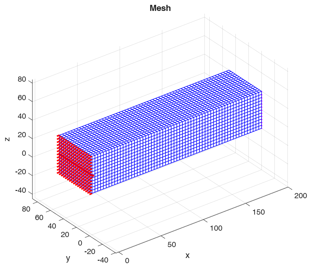
The same cantilever example as in Section 25.1 is used. The coarse mesh has $60\times16\times12$ elements: 11 520 elements, 13 481 nodes and 40 443 equations. The fine mesh has $90\times24\times18$ elements: 38 880 elements, 43 225 nodes and 129 675 equations.

The benefit of vectorization for generation and assembly becomes more pronounced as the mesh is refined. For the coarse mesh, the total computation time is reduced by approximately a factor of 15. For the fine mesh, generation and assembly take only 6.884 s with brick3d_fast, while the direct linear-system solution takes 115.459 s and becomes the dominant computational cost.

05

Preconditioned conjugate gradient method

For large linear-elastic FE systems, after appropriate boundary conditions are imposed, the stiffness matrix is sparse, symmetric and positive definite, so the preconditioned conjugate gradient method (PCG) is well suited. Preconditioning improves conditioning and reduces the number of iterations [1].

The MATLAB implementation uses incomplete Cholesky factorization followed by pcg [2]:

opts.type    = 'ict';
opts.droptol = 1e-3;

L = ichol(K,opts);
[S,flag,relres,iter] = pcg(K,F,1e-6,200,L,L');

ict selects incomplete Cholesky factorization with threshold dropping; droptol = 1e-3 controls the dropping tolerance. $\htmlClass{fea-math-bold-italic}{\boldsymbol{L}}$ and $\htmlClass{fea-math-bold-italic}{\boldsymbol{L}}^{T}$ are used as the two preconditioner factors for pcg.

The incomplete Cholesky factorization provides a sparse approximation of the stiffness matrix:

The factors $\htmlClass{fea-math-bold-italic}{\boldsymbol{L}}$ and $\htmlClass{fea-math-bold-italic}{\boldsymbol{L}}^{T}$ are then used as preconditioners in the PCG algorithm. In simplified form, the preconditioned system may be written as:

Since $\htmlClass{fea-math-bold-italic}{\boldsymbol{L}}\htmlClass{fea-math-bold-italic}{\boldsymbol{L}}^{T}$ approximates $\htmlClass{fea-math-bold-italic}{\boldsymbol{K}}$, the preconditioned system is better conditioned and PCG converges more rapidly.

For the 129 675-equation system, the linear-system solution time drops from about 115.5 s to about 6.7 s, and the total time from about 122.3 s to about 13.3 s. For the present tests, the displacement and stress results from the direct and iterative solvers were identical to the displayed numerical precision.

06

Programs

Use brick3d_fast in place of brick3d with the input and plotting routines from Section 25.1. Keep multiprod.m in the same MATLAB folder. The downloadable program uses the direct solution; the PCG alternative is shown above.

multiprod.m is third-party code by Paolo de Leva and Jinhui Bai; see Section 9.2 and Section 9.5 for source and licensing information.

07

References

1. Y. Saad, Iterative Methods for Sparse Linear Systems, 2nd ed., SIAM, Philadelphia, 2003.
2. MATLAB Documentation, pcg and ichol, MathWorks.