Hyperelastic materials, Mooney-Rivlin material model for nearly incompressible material, Part I

01

Hyperelastic materials

Hyperelastic materials may undergo very large elastic deformations and return to their initial shape after unloading. Elastomers, many polymers, and several biological tissues are common examples. [1], [2], [3]

For an ideal hyperelastic material, the response is history-independent. This means that the stress at a given material point is determined by the current deformation state, not by the sequence of intermediate deformations followed to reach that state. It does not mean that two different loading arrangements necessarily produce the same deformation merely because their final resultant loads are equal. [3]

The constitutive behavior is described through a strain-energy density function $W$. [3] Here, $W$ is the elastic strain energy per unit volume of the initial configuration. In the Total Lagrangian formulation, the constitutive pair consists of the Green–Lagrange strain tensor $\boldsymbol{E}$ and the second Piola–Kirchhoff stress tensor $\boldsymbol{S}$. The stress follows from the variation of stored elastic energy with deformation:

The position vector in the current configuration is related to the initial position and the displacement vector by:

The deformation gradient and the Green-Lagrange strain tensor are:

In three dimensions, the Green–Lagrange strain tensor is written in component form as:

This component notation will be used later when the general three-dimensional constitutive relations are specialized to plane strain.

02

Isotropy and strain invariants

For an isotropic material, there are no preferred directions in the initial configuration. It is therefore natural to express the strain-energy density through the invariants of the right Cauchy–Green tensor, because these scalar quantities are independent of the orientation of the coordinate system: [3]

Because $\boldsymbol{C}$ is symmetric, only six independent components are required in three dimensions. The invariants provide a coordinate-independent description of the deformation and are therefore particularly convenient for isotropic hyperelastic models.

The component notation introduced above will be used in the following expressions for the invariants and their derivatives.

03

Volume change and reduced invariants

The determinant of the deformation gradient gives the local volume ratio:

Thus, $J=1$ indicates no volume change, $J>1$ indicates dilatation, and $J<1$ indicates compression. The third invariant $I_3$ is therefore directly related to local volume change.

The first and second invariants also change during pure dilatation, even though no distortion occurs. To distinguish changes of shape from changes of volume, the reduced invariants are introduced: [1], [3]

Consider a pure dilatation for which $\boldsymbol{C}=c\boldsymbol{I}$. Then:

This shows that the reduced invariants remove the pure volumetric contribution from $I_1$ and $I_2$.

04

Nearly incompressible Mooney-Rivlin model

The two-parameter Mooney–Rivlin model is simple and widely used. It gives satisfactory results for tensile strains up to about 100%, although difficulties may arise in compression. [3] For a nearly incompressible material, the strain-energy density is separated into distortional and volumetric contributions: [3], [4]

The constants $A_{10}$ and $A_{01}$ define the distortional response: changes of shape with the purely volumetric contribution removed. The term containing $K$ represents the energy associated with local volume change. The bulk modulus is large for nearly incompressible materials, so even a small departure of $J$ from unity produces a large volumetric energy penalty. [3]

For small strains, $E\approx6(A_{10}+A_{01})$ in three dimensions, while the corresponding two-dimensional relation used here is $E\approx8(A_{10}+A_{01})$. [3] As $\nu$ approaches 0.5, the bulk modulus tends to infinity and the material approaches the incompressible limit.

For the present numerical example, the volumetric parameter $K=133.33\ {\rm MPa}$ corresponds to $E=4\ {\rm MPa}$ and $\nu=0.495$ through the small-strain bulk-modulus relation. The Mooney-Rivlin constants $A_{10}=0.48\ {\rm MPa}$ and $A_{01}=0.11\ {\rm MPa}$ define the distortional response.

05

PK2 stress and material tangent

The second Piola–Kirchhoff stress follows from the derivative of the strain-energy density with respect to the Green–Lagrange strain. Applying the chain rule to the reduced invariants and $J$ gives:

The material (constitutive) tangent matrix is obtained by differentiating the second Piola–Kirchhoff stress with respect to the Green–Lagrange strain:

Here, $\boldsymbol{D}$ is the three-dimensional $6\times6$ material tangent associated with the Total Lagrangian constitutive pair $\boldsymbol{E}$-$\boldsymbol{S}$. It relates an increment of the six engineering components of Green–Lagrange strain to the corresponding increment of the six second Piola–Kirchhoff stress components. The first and second derivatives follow directly from the chain rule applied to $\bar I_1$, $\bar I_2$, and $J$. [3]

06

Plane-strain specialization

The derivatives of the invariants are first obtained from the general three-dimensional expressions. The plane-strain kinematic constraints are imposed only afterwards. Thus, the out-of-plane strain components that do not belong to the two-dimensional deformation field are set to zero, while the corresponding stress component $S_z$ is still obtained from the full three-dimensional constitutive relation.

The stress component $S_z$ is not set to zero. The three-dimensional constitutive law is retained while the plane-strain kinematic constraint is imposed.

After evaluating the three-dimensional derivatives of the invariants and imposing the plane-strain kinematic constraints, the first derivatives can be written in engineering vector notation as follows:

The second derivatives form symmetric $6\times6$ matrices. For example:

The MoonRiv_strain subprogram computes the complete three-dimensional $6\times6$ constitutive tangent matrix $\boldsymbol{D}$, so that the out-of-plane stress $S_z$ is also obtained. In the stiff subprogram, only rows and columns 1, 2 and 4 of $\boldsymbol{D}$, corresponding to the $x$, $y$ and $xy$ components of the two-dimensional plane-strain problem, are used in the finite-element equations.

D([1 2 4],[1 2 4])

The corresponding plane-stress formulation is presented in Section 18.2, where both a simplified treatment for a nearly incompressible material and an exact enforcement of the plane-stress condition are discussed.

07

MATLAB implementation

The Total Lagrangian Q4 implementation follows the same finite-element sequence used in Section 12.2. At every Gauss point, the Green-Lagrange strain is evaluated and passed to MoonRiv_strain. This subprogram computes $I_1$, $I_2$, $I_3$, the reduced invariants, the PK2 stresses $S_x,S_y,S_z,S_{xy}$, and the $6\times6$ material tangent $\boldsymbol{D}$.

Because the material is hyperelastic, the stresses are calculated directly from the current deformation through the strain-energy density function; no stress-history update is required.

% Green-Lagrange strains:
E=B*S+B_nl*S;

% constitutive calculation:
MoonRiv_strain

% plane-strain material tangent:
D2=D([1 2 4],[1 2 4]);

% store strains:
strnt(ig,:,istep+1)=E';

The RMS displacement correction used as convergence measure is evaluated over all equations:

error=sqrt(dS'*dS/neq);

08

Numerical example

The example is a perforated plate modeled in plane strain with 767 nodes and 685 isoparametric Q4 elements. The material constants are:

The loading is increased incrementally to $F=160\ {\rm N}$, and symmetry conditions are used. In ANSYS, the same Mooney–Rivlin constants $A_{10}$ and $A_{01}$ are supplied together with the incompressibility parameter $d$. For the volumetric energy convention used in this example, $d=2/K=0.015\ {\rm MPa}^{-1}$. [1]

ANSYS output provides Cauchy stresses and Hencky strains in the global coordinate frame. [1] The comparisons below use displacements as the primary global response and show corresponding displacement and strain maps on the same plotting geometry.

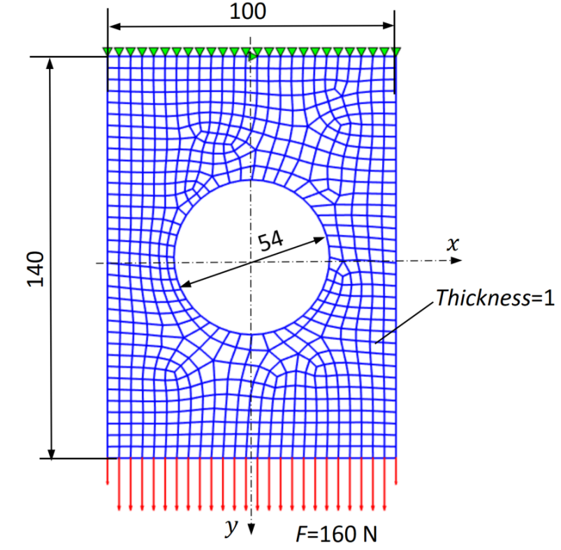
The standard displacement formulation converges slowly and uses under-relaxation:

sr=0.167;
S=S-dS*sr;

The slow convergence is mainly associated with the nearly incompressible character of the material. The volumetric stiffness is much larger than the distortional stiffness, which makes the standard displacement formulation numerically difficult. An under-relaxation factor is therefore used here to improve robustness. In Section 18.3, this difficulty will be treated more effectively by Selective Reduced Integration, in which the volumetric and distortional contributions are integrated differently.

09

Displacement comparison

The force-displacement curve obtained with the MATLAB program is compared with ANSYS. In the ANSYS finite-strain hyperelastic constitutive description, the strain-energy function is expressed using deformation quantities referred to the undeformed configuration. [1] This is consistent with the Total Lagrangian formulation adopted in the present MATLAB program.

The displacement maps are presented on the undeformed geometry so that the MATLAB and ANSYS results can be compared directly using the same visual representation. This plotting choice is consistent with the adopted Total Lagrangian description, but is not imposed by it.

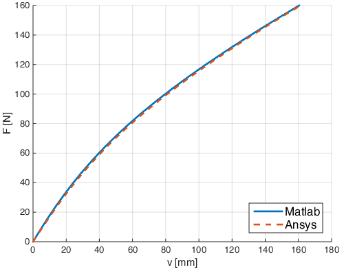
The maximum downward displacements are $v_{\max}=159.41\ {\rm mm}$ in MATLAB and $v_{\max}=161.23\ {\rm mm}$ in ANSYS.

10

Strain comparison

The MATLAB program stores Green–Lagrange strains. For comparison with the logarithmic strain output from ANSYS, the Hencky strain is evaluated during postprocessing:

The following maps compare the vertical strain component in the global coordinate frame. The MATLAB Green–Lagrange result is shown together with the MATLAB and ANSYS Hencky-strain results. All three maps are presented on the undeformed geometry for a direct visual comparison.

11

Programs and references

The MATLAB program, the Hencky-strain postprocessor, and the ANSYS macro used for this example can be downloaded below.

References

1. [1]Ansys Inc., ANSYS Mechanical APDL Theory Reference, Release 2026 R1, 2026.
2. [2]Hyperelastic material, Wikipedia.
3. [3]N.-H. Kim, Introduction to Non-Linear Finite Element Analysis, Springer, 2015.
4. [4]J. Bonet and R. D. Wood, Nonlinear Continuum Mechanics for Finite Element Analysis, Cambridge University Press, 1997.