01
Formulation and hypotheses
Hyperelastic materials may undergo large recoverable elastic strains. Elastomers such as rubber, many polymers, and several biological tissues belong to this category. [2], [3]
For an ideal hyperelastic material, the response is history-independent: the stress state at a material point is determined by the current deformation, rather than by the deformation history used to reach it. [3]
The elastic behavior is described by the strain-energy density , expressed per unit volume of the initial configuration. The Total Lagrangian formulation introduced in Section 18.1 is retained. Its constitutive pair consists of the Green-Lagrange strain tensor and the second Piola-Kirchhoff stress tensor :
The nearly incompressible Mooney-Rivlin energy is:
02
Plane-stress condition and invariants
For a plane-stress state, the Green-Lagrange strain and second Piola-Kirchhoff stress tensors have the forms:
The out-of-plane strain , however, is generally non-zero. The right Cauchy-Green tensor is:
Using the component notation above, the invariants are:
03
Out-of-plane strain from the incompressibility approximation
For the plane-stress state, the out-of-plane stress is zero, , whereas the out-of-plane strain is generally non-zero. For an exact plane-stress solution, should be determined from the condition using the complete hyperelastic constitutive relation.
In the present nearly incompressible formulation, a simpler approximation is adopted. Since Poisson's ratio is very close to , the volume change is expected to be very small; therefore:
In the calculations, the condition imposed is:
This condition is an approximation justified by the nearly incompressible material and is not a general consequence of plane stress. Since:
the imposed approximation gives:
The three-dimensional deformation gradient is:
For the two-dimensional plane-stress kinematics, , while the thickness stretch remains unknown. Hence:
Because , the unknown out-of-plane component satisfies . The condition gives:
Therefore:
Since is imposed, its first and second derivatives vanish in this formulation:
04
Symbolic derivatives and MoonRiv_stress
Because is expressed in terms of the in-plane components through the incompressibility condition , the analytical expressions of the first and second derivatives of and become cumbersome. The MATLAB Symbolic Math Toolbox is therefore used to evaluate these derivatives automatically. The resulting expressions are then transferred to the MoonRiv_stress subprogram.
The symbolic program first defines from the incompressibility constraint, constructs the right Cauchy-Green tensor , evaluates and , and finally differentiates them with respect to , , and . The derivatives with respect to the Green-Lagrange strains are then obtained using .
clear
clc
syms Cxx Cyy Czz Cxy real
Czz=1/(Cxx*Cyy-Cxy^2);
C=[Cxx Cxy 0; Cxy Cyy 0; 0 0 Czz];

I1=trace(C)
I2=1/2*(trace(C)^2-trace(C^2)); I2=expand(I2)

I1E=[diff(I1,Cxx); diff(I1,Cyy); 0; diff(I1,Cxy); 0; 0]*2
I2E=[diff(I2,Cxx); diff(I2,Cyy); 0; diff(I2,Cxy); 0; 0]*2

zr=zeros(6,1);
I1EE=[diff(I1E,Cxx) diff(I1E,Cyy) zr diff(I1E,Cxy) zr zr]*2
I2EE=[diff(I2E,Cxx) diff(I2E,Cyy) zr diff(I2E,Cxy) zr zr]*2
The MATLAB programs used in this section are very similar to those of Section 18.1. The main change is the replacement of the MoonRiv_strain subprogram by MoonRiv_stress. In the plane-stress formulation, the out-of-plane strain is first obtained from the incompressibility approximation . This makes a function of the in-plane strain components, and therefore the derivatives of the invariants and differ from those used in the plane-strain case. The subprogram MoonRiv_stress contains these new first- and second-derivative expressions and uses them to compute the second Piola-Kirchhoff stresses and the constitutive tangent matrix.
Apart from this constitutive modification, the finite-element structure of the program remains essentially unchanged.
05
MATLAB implementation and convergence
The Total Lagrangian Q4 assembly follows the same sequence used in Sections 12.2 and 18.1. The Green-Lagrange strains are evaluated at every Gauss point, the constitutive response is obtained from MoonRiv_stress, and the element internal-force vector and tangent stiffness matrix are assembled into the corresponding global positions.
Because the material is hyperelastic, the stresses are calculated directly from the current deformation through the strain-energy density function; no stress-history update is required.
% Green-Lagrange strains:
ex =ux+ux^2/2+vx^2/2;
ey =vy+uy^2/2+vy^2/2;
exy=uy+vx+ux*uy+vx*vy;

% constitutive calculation:
MoonRiv_stress

% store stresses:
sigmt(ig,:,istep+1)=[sx sy sz sxy];

% store strains:
strnt(ig,:,istep+1)=[ex,ey,ez,exy];
In the present plane-stress approximation, the out-of-plane strain is determined by imposing . Consequently, the volumetric contribution to the strain-energy density vanishes within the imposed approximation, while the response is governed mainly by the distortional part. The large difference between volumetric and distortional stiffness that caused the slow convergence in the plane-strain formulation of Section 18.1 is therefore greatly reduced, and the Newton iteration converges much more rapidly. This conclusion applies specifically to the present approximation and should not be interpreted as a general property of every plane-stress hyperelastic formulation.
For a nearly incompressible material, with Poisson's ratio very close to 0.5, the approximation was adopted in the formulation presented above. This leads to a particularly simple plane-stress treatment and requires only minor modifications of the program presented in Section 18.1. A rigorous enforcement of the plane-stress condition, together with a comparison of the numerical results and the corresponding MATLAB programs, is presented in the following addendum.
06
Numerical example
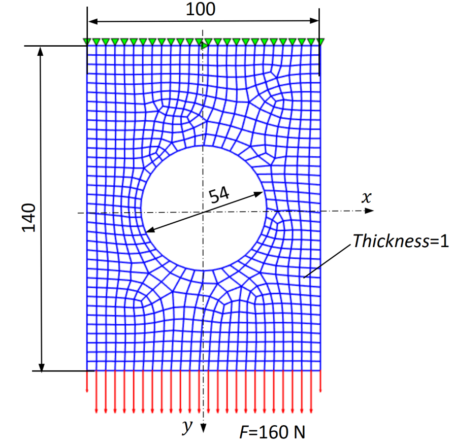
A perforated plate is analyzed in plane stress. The mesh has 767 nodes and 685 isoparametric Q4 elements. The plate thickness is , and the total applied force is .
For the present numerical example, the volumetric parameter corresponds to and through the small-strain bulk-modulus relation. The Mooney-Rivlin constants and define the distortional response.
ANSYS uses the incompressibility parameter instead of the bulk modulus for this material definition. With the volumetric energy convention used here:
The ANSYS finite-strain hyperelastic reference model uses the same geometry, mesh, loading, and material constants. [1]
07
Displacement comparison
The vertical displacement of the central node on the loaded side is plotted against the applied force. The MATLAB and ANSYS curves are in very good agreement.
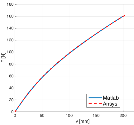
At the final load, the maximum downward displacements are in MATLAB and approximately in ANSYS.
The displacement maps below are shown on the deformed configuration. The two distributions are nearly identical.
08
Green-Lagrange and Hencky strains
The main MATLAB program stores the Green-Lagrange strain. For comparison with the logarithmic output from ANSYS, the Hencky strain is evaluated in a separate postprocessing program:
ANSYS reports Hencky strains in the global coordinate frame. [1] The following maps compare the vertical component: MATLAB Green-Lagrange strain, MATLAB Hencky strain, and ANSYS Hencky strain. The maps are presented on the undeformed configuration, consistently with the Total Lagrangian description adopted in the present formulation.
09
PK2 and Cauchy stresses
The constitutive calculation provides the second Piola-Kirchhoff stress . ANSYS reports Cauchy stresses in the global coordinate frame. [1] The usual transformation is:
In the present nearly incompressible plane-stress approximation, is imposed when determining the out-of-plane strain. Therefore, the transformation reduces here to:
The maps below compare the vertical second Piola-Kirchhoff stress calculated in MATLAB with the MATLAB and ANSYS Cauchy stresses. All components are referred to the global coordinate frame.
10
Out-of-plane Hencky strain
The final comparison concerns the out-of-plane Hencky strain. In MATLAB it is evaluated from the thickness component of the right Cauchy-Green tensor:
The corrected MATLAB postprocessing gives and . The corresponding ANSYS map spans approximately to . The tensile maximum is close, while the most compressive local value shows a larger difference.
ADDENDUM
Addendum — Exact enforcement of the plane-stress condition
by Chiara
01. Exact plane stress versus the approximation
The formulation developed above uses the approximation , which is especially attractive for a nearly incompressible material. Exact plane stress, however, is defined by the vanishing out-of-plane stress:
When the transverse shear stresses are absent, this condition is equivalent to . It is important to distinguish the two conditions:
The first condition represents exact incompressibility, whereas the second represents exact plane stress. A plane-stress state does not, by itself, imply .
02. Local Newton solution for the out-of-plane strain
In the exact formulation, the out-of-plane Green–Lagrange strain is determined at each Gauss point as the local unknown that satisfies:
A local Newton iteration is used:
The quantity is a local constitutive variable. It is not an additional nodal degree of freedom, so the global finite-element system retains the same size.
The incompressibility relation provides an excellent initial estimate for this local iteration. With:
the local volume ratio satisfies:
Setting only for the initial estimate gives:
For a nearly incompressible material, this estimate is already close to the exact solution and makes the local constitutive iteration efficient and robust.
The local MATLAB sequence is:
ia=[1 2 4];

Cxx=2*ex+1; Cyy=2*ey+1; Cxy=exy;
ez=(1/(Cxx*Cyy-Cxy^2)-1)/2;

tolz=1e-10;
iterzmax=25;

for iterz=1:iterzmax
    MoonRiv_exact_stress
    if abs(sz)<tolz, break, end
    ez=ez-sz/D(3,3);
end
Here, sz is , D(3,3) is , and the initial value of ez follows from . The converged value is the local solution that satisfies .
03. Consistent plane-stress tangent
The constitutive calculation remains three-dimensional throughout the local Newton iteration. The stresses and the complete three-dimensional tangent are reevaluated until is satisfied.
By separating the in-plane components from the transverse one, the constitutive relation may be written in block form as
Using engineering-component vectors written as columns:
where denotes the set of active in-plane components. The incremental constitutive equations can be partitioned as:
Exact plane stress requires . Therefore:
and the consistent condensed plane-stress tangent becomes:
The effect of is therefore condensed into the in-plane response, not neglected, and no additional global degree of freedom is introduced.
04. Modification of stiff
The separate MATLAB package retains the simplified formulation and permits selection of the desired treatment:
iplane=2;    % 1 - J=1 approximation
             % 2 - exact plane stress, Sz=0
With iplane=1, the program uses the simplified formulation. With iplane=2, it solves the local equation and forms the condensed tangent. The complete constitutive part displayed on the site is:
% constitutive calculation:
ia=[1 2 4];

if iplane==1

    MoonRiv_stress
    Dps=D(ia,ia);

elseif iplane==2

    Cxx=2*ex+1; Cyy=2*ey+1; Cxy=exy;
    ez=(1/(Cxx*Cyy-Cxy^2)-1)/2;

    tolz=1e-10;
    iterzmax=25;

    for iterz=1:iterzmax
        MoonRiv_exact_stress
        if abs(sz)<tolz, break, end
        ez=ez-sz/D(3,3);
    end

    Dps=D(ia,ia)-D(ia,3)*(D(3,3)\D(3,ia));

    Jt=Jt+sqrt(I3);

end
05. Mean volume ratio
For iplane=2, the program accumulates the local volume ratio at all four Gauss points of every element. At the end of the analysis it reports:
if iplane==2, disp(['J_mean = ',num2str(Jt/4/nel)]), endNo corresponding value is displayed for iplane=1, because that formulation imposes directly.
06. Numerical comparison
For the perforated-plate example, the simplified and exact formulations give the following final results:
| Formulation | Condition | ||
|---|---|---|---|
| Simplified | imposed | ||
| Exact plane stress |
The displacement difference is approximately , or . The exact formulation gives , corresponding to an average volumetric departure of about . Thus, the simplified condition gives a close structural response for this nearly incompressible example, while the exact formulation reveals the small but non-zero volume change required to satisfy .
07. Final distinction
The distinction can be summarized as:
The comparison also illustrates why the approximation is so attractive in a nearly incompressible material: it captures the structural response with good accuracy while avoiding the local nonlinear solution required by the exact plane-stress condition.
11
Programs and references
The Q4 analysis programs, Hencky-strain postprocessor, Cauchy-stress postprocessor, and ANSYS macro used for this example can be downloaded below.
References
- [1]Ansys Inc., ANSYS Mechanical APDL Theory Reference, Release 2026 R1, 2026.
- [2]Hyperelastic material, Wikipedia.
- [3]N.-H. Kim, Introduction to Non-Linear Finite Element Analysis, Springer, 2015.