18.3. Mooney-Rivlin model for nearly incompressible materials, Selective Reduced Integration

Formulation and hypotheses

StrainLarge

DisplacementLarge

MaterialNonlinear elastic

Material symmetryIsotropic

Stress statePlane strain

The nearly incompressible plane-strain formulation presented in Section 18.1 converges slowly when the standard displacement formulation and full $2\times2$ Gauss integration are used. As Poisson's ratio approaches $0.5$ , the bulk modulus becomes much larger than the distortional stiffness, and the finite element becomes excessively constrained by the nearly isochoric response. This numerical effect is known as volumetric locking [1].

The idea of Selective Reduced Integration is to under-integrate the volumetric contribution to the element stiffness, thereby relaxing the excessive volumetric constraint responsible for locking. The distortional part is still integrated with the standard rule:

\boldsymbol{k}_{\rm dist}:\quad 2\times2\ \text{Gauss rule},\qquad \boldsymbol{k}_{\rm vol}:\quad 1\times1\ \text{Gauss rule}

This treatment improves the convergence of the present problem, although it should not be interpreted as a guarantee that every convergence difficulty disappears in every nearly incompressible problem.

Distortional and volumetric contributions

The strain-energy density of the nearly incompressible Mooney-Rivlin material is separated into distortional and volumetric parts:

\boxed{W=W_{\rm dist}+W_{\rm vol}}

W_{\rm dist}=A_{10}(\bar I_1-3)+A_{01}(\bar I_2-3),\qquad W_{\rm vol}=\frac{K}{2}(J-1)^2

Here $K$ is the scalar bulk modulus. It must not be confused with the global stiffness matrix $\boldsymbol{K}$ . The separation of $W$ produces separate distortional and volumetric stress and tangent contributions, allowing different quadrature rules to be applied to the two parts.

The second Piola–Kirchhoff stresses are:

\boldsymbol{S}_{\rm dist}=\frac{\partial W_{\rm dist}}{\partial\boldsymbol{E}}=A_{10}\frac{\partial\bar I_1}{\partial\boldsymbol{E}}+A_{01}\frac{\partial\bar I_2}{\partial\boldsymbol{E}}

\boldsymbol{S}_{\rm vol}=\frac{\partial W_{\rm vol}}{\partial\boldsymbol{E}}=K(J-1)\frac{\partial J}{\partial\boldsymbol{E}}

The corresponding material tangent contributions are:

\boldsymbol{D}_{\rm dist}=A_{10}\frac{\partial^2\bar I_1}{\partial\boldsymbol{E}^2}+A_{01}\frac{\partial^2\bar I_2}{\partial\boldsymbol{E}^2}

\boldsymbol{D}_{\rm vol}=K(J-1)\frac{\partial^2J}{\partial\boldsymbol{E}^2}+K\frac{\partial J}{\partial\boldsymbol{E}}\left(\frac{\partial J}{\partial\boldsymbol{E}}\right)^T

The element stiffness matrix is consequently written as:

\boldsymbol{k}_{\rm el}=\boldsymbol{k}_{\rm dist}+\boldsymbol{k}_{\rm vol}

Selective Reduced Integration

The distortional contribution is evaluated at the four Gauss points of the standard $2\times2$ rule. Each of these points has weight 1. The volumetric contribution is evaluated only at the element centre, using the $1\times1$ rule. In one dimension the central point has weight 2; therefore the total two-dimensional weight is:

w_G=2\times2=4

Gauss points and weights for one- and two-point integration — **Figure 1.** Gauss points and weights used to construct the $2\times2$ and $1\times1$ quadrature rules.

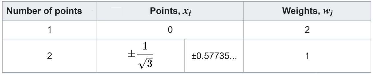
The subscript $g=1,\ldots,4$ denotes quantities evaluated at the four $2\times2$ Gauss points, whereas the subscript $0$ denotes quantities evaluated at the element centre for the $1\times1$ rule.

\begin{aligned} \boldsymbol{k}_{\rm el}={}&h\sum_{g=1}^{4}\left[\boldsymbol{B}_g^T\boldsymbol{D}_{{\rm dist},g}\boldsymbol{B}_g+S_{x,g}\boldsymbol{G}_{x,g}+S_{y,g}\boldsymbol{G}_{y,g}+S_{xy,g}\boldsymbol{G}_{xy,g}\right]\det\boldsymbol{J}_g\\ &+4h\left[\boldsymbol{B}_0^T\boldsymbol{D}_{{\rm vol},0}\boldsymbol{B}_0+S_{x,0}\boldsymbol{G}_{x,0}+S_{y,0}\boldsymbol{G}_{y,0}+S_{xy,0}\boldsymbol{G}_{xy,0}\right]\det\boldsymbol{J}_0 \end{aligned}

The factor 4 in the second line is the complete weight of the one-point rule.

Stress and tangent evaluation

The distortional stresses and tangent contributions are evaluated at the four $2\times2$ Gauss points. The volumetric stress and tangent contribution are evaluated only at the element centre using the $1\times1$ rule and are then combined with the distortional contribution at each of the four Gauss points.

Thus, the total second Piola–Kirchhoff stress stored at Gauss point $g$ is:

\boxed{\boldsymbol{S}_g=\boldsymbol{S}_{{\rm dist},g}+\boldsymbol{S}_{{\rm vol},0},\qquad g=1,\ldots,4}

The distinction is important: the element stiffness is integrated with two different quadrature rules, whereas the total stress reported at each of the four Gauss points is formed by combining the local distortional value with the single central volumetric value.

The global finite-element equations are assembled from the element contributions:

\boldsymbol{K}=\mathop{\mathcal A}_{el=1}^{n_{el}}\left(\boldsymbol{k}_{\rm el}\right),\qquad \boldsymbol{F}_{\rm int}=\mathop{\mathcal A}_{el=1}^{n_{el}}\left(\boldsymbol{f}_{\rm el}\right)

MATLAB implementation

The stiff routine from Section 18.1 is effectively split into distortional and volumetric calculations. The program stiff_distortion uses the four Gauss points and calls MoonRiv_distortion. The program stiff_bulk uses the element centre and calls MoonRiv_bulk. The complete contributions are assembled in the common global system.

The short coordinating routine stiff is copied below. It simply calls stiff_distortion and stiff_bulk, which compute the distortional and volumetric contributions, respectively.

stiff.m

%*** stiff ***
% Gauss points
st=[1  -1  -1   1
    1   1  -1  -1]*sqrt(3)/3;
F=zeros(neq,1);
K=zeros(neq);
stiff_distortion
stiff_bulk
% Constraints
loc=2*(cond(:,1)-1)+cond(:,2);
K(loc,:  )=0; K(:  ,loc)=0; F(loc,:  )=0;
K(loc,loc)=eye(length(loc));
% Concentrated force
loc=2*(forze(:,1)-1)+forze(:,2);
F(loc)=F(loc)-forze(:,3)*istep/nstep;

Because the material is hyperelastic, the stresses are evaluated directly from the current deformation through the strain-energy density function; no stress-history update is required. The postprocessor converts the stored second Piola–Kirchhoff stresses to Cauchy stresses through:

\boldsymbol{\sigma}=\frac{1}{J}\boldsymbol{F}\boldsymbol{S}\boldsymbol{F}^T

The nonlinear convergence norm is evaluated over all equations:

\mathrm{error}=\sqrt{\frac{\Delta\boldsymbol{S}^T\Delta\boldsymbol{S}}{n_{eq}}}

Numerical example

The same perforated plate used in Sections 18.1 and 18.2 is analyzed in plane strain. The mesh has 767 nodes and 685 Q4 elements. The plate thickness is $h=1\ {\rm mm}$ , and the applied force is $F=160\ {\rm N}$ .

For the present example, the volumetric parameter $K=133.33\ {\rm MPa}$ corresponds to $E=4\ {\rm MPa}$ and $\nu=0.495$ through the small-strain bulk-modulus relation. The Mooney-Rivlin constants $A_{10}=0.48\ {\rm MPa}$ and $A_{01}=0.11\ {\rm MPa}$ define the distortional response.

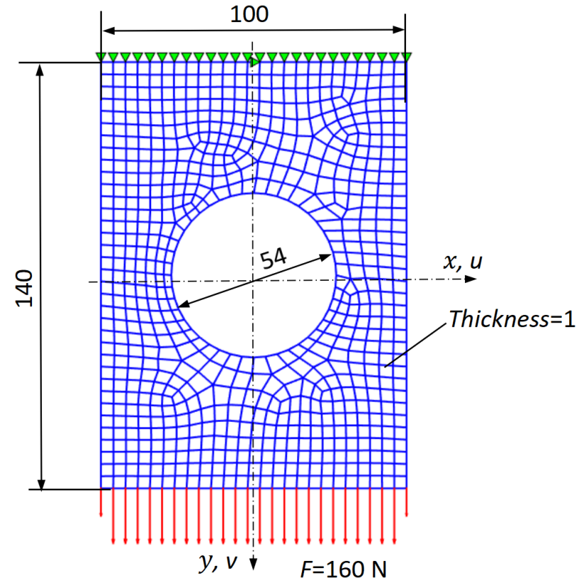
Perforated plate, loading, boundary conditions, dimensions, and Q4 mesh — **Figure 2.** Perforated plate, loading, boundary conditions, dimensions, and Q4 finite-element mesh.

The Selective Reduced Integration formulation converges much more rapidly than the fully integrated plane-strain formulation of Section 18.1. This improvement results from reducing the volumetric locking produced by the standard displacement formulation. The displacements are also closer to the ANSYS results.

Displacement comparison

The following maps compare the MATLAB and ANSYS displacement components. The MATLAB analysis gives $u_{\min}=-24.8447\ {\rm mm}$ , $u_{\max}=25.9957\ {\rm mm}$ , and $v_{\min}=-161.1509\ {\rm mm}$ . The corresponding ANSYS values are approximately $u_{\min}=-24.8427\ {\rm mm}$ , $u_{\max}=25.9955\ {\rm mm}$ , and $v_{\min}=-161.231\ {\rm mm}$ .

MATLAB horizontal displacement with turbo colormap — **Figure 3a.** MATLAB horizontal displacement $u$ .

**Figure 3b.** ANSYS horizontal displacement $u$ .

MATLAB vertical displacement with turbo colormap — **Figure 4a.** MATLAB vertical displacement $v$ .

**Figure 4b.** ANSYS vertical displacement $v$ .

Cauchy-stress comparisons

The comparison includes all in-plane and out-of-plane Cauchy-stress components. The MATLAB maps below were regenerated from the authoritative MoonRiv_3 package with turbo(16); the ANSYS maps are retained unchanged. All stresses are expressed in MPa.

MATLAB Cauchy stress sigma x with turbo colormap — **Figure 5a.** MATLAB $\sigma_x$ : min $-1.2118$ , max $0.33414$ .

ANSYS Cauchy stress sigma x — **Figure 5b.** ANSYS $\sigma_x$ : min $-1.16208$ , max $0.294889$ .

MATLAB Cauchy stress sigma y with turbo colormap — **Figure 6a.** MATLAB $\sigma_y$ : min $0.11803$ , max $16.3096$ .

ANSYS Cauchy stress sigma y — **Figure 6b.** ANSYS $\sigma_y$ : min $0.172396$ , max $14.7891$ .

MATLAB Cauchy stress sigma z with turbo colormap — **Figure 7a.** MATLAB $\sigma_z$ : min $-0.57222$ , max $3.1431$ .

ANSYS Cauchy stress sigma z — **Figure 7b.** ANSYS $\sigma_z$ : min $-0.601061$ , max $3.19738$ .

MATLAB Cauchy shear stress tau xy with turbo colormap — **Figure 8a.** MATLAB $\tau_{xy}$ : min $-1.1697$ , max $1.6739$ .

ANSYS Cauchy shear stress tau xy — **Figure 8b.** ANSYS $\tau_{xy}$ : min $-1.01436$ , max $1.03491$ .

Force-balance verification

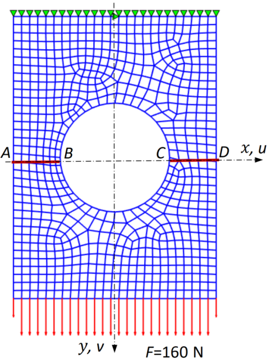
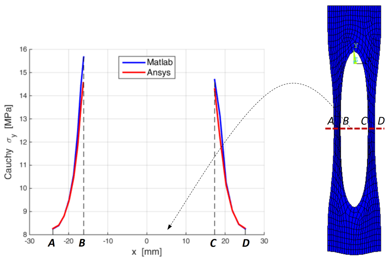
A useful final verification is obtained by integrating the vertical Cauchy stress along the two line segments $AB$ and $CD$ :

\boxed{F=h\int_{AB+CD}\sigma_y\,dx}

The integration is performed along the deformed lines because the Cauchy stresses act on the current configuration. For the MATLAB solution, the resultant of the Cauchy stresses $\sigma_y$ is $162.39\ {\rm N}$ , compared with the applied force $F=160\ {\rm N}$ .

Deformed perforated plate and the AB and CD integration paths — **Figure 9.** Deformed lines $AB$ and $CD$ used for the force-balance verification.

MATLAB and ANSYS sigma y distributions along AB and CD — **Figure 10.** MATLAB and ANSYS distributions of the Cauchy stress $\sigma_y$ along $AB+CD$ .

Programs and reference

The complete MATLAB package contains the Q4 mesh, Selective Reduced Integration routines, Mooney-Rivlin constitutive subprograms, Cauchy-stress conversion, plotting programs, and a README.

MATLABMooney-Rivlin Q4 plane-strain SRI programsMATLAB programs, mesh data, and READMEDOWNLOAD ZIP

Reference

[1]N.-H. Kim, Introduction to Non-Linear Finite Element Analysis, Springer, 2015.