01
Element and hypotheses The four-node bilinear isoparametric quadrilateral is introduced following the standard finite element formulation presented by Felippa [1] . The element has four nodes and two translational DOFs per node.
Strain Small
Displacement Small
Material Linear elastic
Stress state Plane stress
f e l = k e l u e l
\boldsymbol{f}_{el}=\boldsymbol{k}_{el}\boldsymbol{u}_{el}
f e l = k e l u e l f e l = { X 1 Y 1 X 2 Y 2 X 3 Y 3 X 4 Y 4 } , u e l = { u 1 v 1 u 2 v 2 u 3 v 3 u 4 v 4 }
\boldsymbol{f}_{el}=
\begin{Bmatrix}
X_1\\Y_1\\X_2\\Y_2\\X_3\\Y_3\\X_4\\Y_4
\end{Bmatrix},
\qquad
\boldsymbol{u}_{el}=
\begin{Bmatrix}
u_1\\v_1\\u_2\\v_2\\u_3\\v_3\\u_4\\v_4
\end{Bmatrix}
f e l = ⎩ ⎨ ⎧ X 1 Y 1 X 2 Y 2 X 3 Y 3 X 4 Y 4 ⎭ ⎬ ⎫ , u e l = ⎩ ⎨ ⎧ u 1 v 1 u 2 v 2 u 3 v 3 u 4 v 4 ⎭ ⎬ ⎫ Here f e l \boldsymbol{f}_{el} f e l u e l \boldsymbol{u}_{el} u e l k e l \boldsymbol{k}_{el} k e l
02
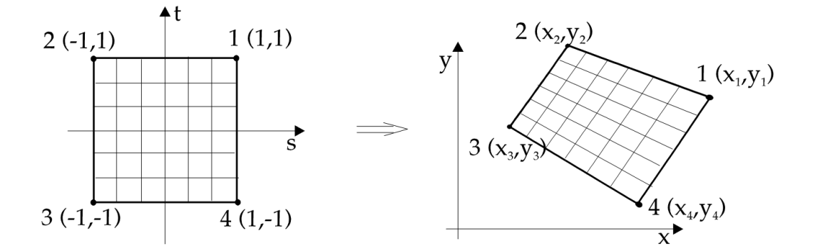
Natural coordinates and interpolation Figure 1. The four-node element in the natural ( s , t ) (s,t) ( s , t ) ( x , y ) (x,y) ( x , y ) The displacement field is interpolated from the nodal values:
{ u ( s , t ) v ( s , t ) } = [ N u N v ] u e l = [ N 1 ( s , t ) 0 N 2 ( s , t ) 0 N 3 ( s , t ) 0 N 4 ( s , t ) 0 0 N 1 ( s , t ) 0 N 2 ( s , t ) 0 N 3 ( s , t ) 0 N 4 ( s , t ) ] u e l
\begin{Bmatrix}u(s,t)\\v(s,t)\end{Bmatrix}
=\begin{bmatrix}\boldsymbol{N}_u\\\boldsymbol{N}_v\end{bmatrix}\boldsymbol{u}_{el}
=
\begin{bmatrix}
N_1(s,t)&0&N_2(s,t)&0&N_3(s,t)&0&N_4(s,t)&0\\
0&N_1(s,t)&0&N_2(s,t)&0&N_3(s,t)&0&N_4(s,t)
\end{bmatrix}\boldsymbol{u}_{el}
{ u ( s , t ) v ( s , t ) } = [ N u N v ] u e l = [ N 1 ( s , t ) 0 0 N 1 ( s , t ) N 2 ( s , t ) 0 0 N 2 ( s , t ) N 3 ( s , t ) 0 0 N 3 ( s , t ) N 4 ( s , t ) 0 0 N 4 ( s , t ) ] u e l The same interpolation functions are used for the geometry:
{ x ( s , t ) y ( s , t ) } = [ N u N v ] x e l = [ N 1 ( s , t ) 0 N 2 ( s , t ) 0 N 3 ( s , t ) 0 N 4 ( s , t ) 0 0 N 1 ( s , t ) 0 N 2 ( s , t ) 0 N 3 ( s , t ) 0 N 4 ( s , t ) ] x e l
\begin{Bmatrix}x(s,t)\\y(s,t)\end{Bmatrix}
=\begin{bmatrix}\boldsymbol{N}_u\\\boldsymbol{N}_v\end{bmatrix}\boldsymbol{x}_{el}
=
\begin{bmatrix}
N_1(s,t)&0&N_2(s,t)&0&N_3(s,t)&0&N_4(s,t)&0\\
0&N_1(s,t)&0&N_2(s,t)&0&N_3(s,t)&0&N_4(s,t)
\end{bmatrix}\boldsymbol{x}_{el}
{ x ( s , t ) y ( s , t ) } = [ N u N v ] x e l = [ N 1 ( s , t ) 0 0 N 1 ( s , t ) N 2 ( s , t ) 0 0 N 2 ( s , t ) N 3 ( s , t ) 0 0 N 3 ( s , t ) N 4 ( s , t ) 0 0 N 4 ( s , t ) ] x e l x e l = [ x 1 y 1 x 2 y 2 x 3 y 3 x 4 y 4 ] T
\boldsymbol{x}_{el}
=\begin{bmatrix}x_1&y_1&x_2&y_2&x_3&y_3&x_4&y_4\end{bmatrix}^{T}
x e l = [ x 1 y 1 x 2 y 2 x 3 y 3 x 4 y 4 ] T The four bilinear interpolation functions are:
N 1 ( s , t ) = ( 1 + s ) ( 1 + t ) 4 , N 2 ( s , t ) = ( 1 − s ) ( 1 + t ) 4
N_1(s,t)=\frac{(1+s)(1+t)}{4},\qquad
N_2(s,t)=\frac{(1-s)(1+t)}{4}
N 1 ( s , t ) = 4 ( 1 + s ) ( 1 + t ) , N 2 ( s , t ) = 4 ( 1 − s ) ( 1 + t ) N 3 ( s , t ) = ( 1 − s ) ( 1 − t ) 4 , N 4 ( s , t ) = ( 1 + s ) ( 1 − t ) 4 , s , t ∈ [ − 1 , 1 ]
N_3(s,t)=\frac{(1-s)(1-t)}{4},\qquad
N_4(s,t)=\frac{(1+s)(1-t)}{4},
\qquad s,t\in[-1,1]
N 3 ( s , t ) = 4 ( 1 − s ) ( 1 − t ) , N 4 ( s , t ) = 4 ( 1 + s ) ( 1 − t ) , s , t ∈ [ − 1 , 1 ] 03
Strains and Jacobian The engineering strain vector is:
ε = { ε x ε y γ x y } = { ∂ u ∂ x ∂ v ∂ y ∂ u ∂ y + ∂ v ∂ x }
\boldsymbol{\varepsilon}
=\begin{Bmatrix}\varepsilon_x\\\varepsilon_y\\\gamma_{xy}\end{Bmatrix}
=\begin{Bmatrix}
\dfrac{\partial u}{\partial x}\\[4pt]
\dfrac{\partial v}{\partial y}\\[4pt]
\dfrac{\partial u}{\partial y}+\dfrac{\partial v}{\partial x}
\end{Bmatrix}
ε = ⎩ ⎨ ⎧ ε x ε y γ x y ⎭ ⎬ ⎫ = ⎩ ⎨ ⎧ ∂ x ∂ u ∂ y ∂ v ∂ y ∂ u + ∂ x ∂ v ⎭ ⎬ ⎫ ε = [ 1 0 0 0 0 1 ] { ∂ u ∂ x ∂ u ∂ y } + [ 0 0 0 1 1 0 ] { ∂ v ∂ x ∂ v ∂ y }
\boldsymbol{\varepsilon}
=
\begin{bmatrix}1&0\\0&0\\0&1\end{bmatrix}
\begin{Bmatrix}\dfrac{\partial u}{\partial x}\\[3pt]\dfrac{\partial u}{\partial y}\end{Bmatrix}
+
\begin{bmatrix}0&0\\0&1\\1&0\end{bmatrix}
\begin{Bmatrix}\dfrac{\partial v}{\partial x}\\[3pt]\dfrac{\partial v}{\partial y}\end{Bmatrix}
ε = 1 0 0 0 0 1 ⎩ ⎨ ⎧ ∂ x ∂ u ∂ y ∂ u ⎭ ⎬ ⎫ + 0 0 1 0 1 0 ⎩ ⎨ ⎧ ∂ x ∂ v ∂ y ∂ v ⎭ ⎬ ⎫ Cartesian derivatives are obtained from derivatives with respect to the natural coordinates:
{ ∂ u ∂ x ∂ u ∂ y } = J − 1 { ∂ u ∂ s ∂ u ∂ t } , { ∂ v ∂ x ∂ v ∂ y } = J − 1 { ∂ v ∂ s ∂ v ∂ t }
\begin{Bmatrix}\dfrac{\partial u}{\partial x}\\[3pt]\dfrac{\partial u}{\partial y}\end{Bmatrix}
=\boldsymbol{J}^{-1}
\begin{Bmatrix}\dfrac{\partial u}{\partial s}\\[3pt]\dfrac{\partial u}{\partial t}\end{Bmatrix},
\qquad
\begin{Bmatrix}\dfrac{\partial v}{\partial x}\\[3pt]\dfrac{\partial v}{\partial y}\end{Bmatrix}
=\boldsymbol{J}^{-1}
\begin{Bmatrix}\dfrac{\partial v}{\partial s}\\[3pt]\dfrac{\partial v}{\partial t}\end{Bmatrix}
⎩ ⎨ ⎧ ∂ x ∂ u ∂ y ∂ u ⎭ ⎬ ⎫ = J − 1 ⎩ ⎨ ⎧ ∂ s ∂ u ∂ t ∂ u ⎭ ⎬ ⎫ , ⎩ ⎨ ⎧ ∂ x ∂ v ∂ y ∂ v ⎭ ⎬ ⎫ = J − 1 ⎩ ⎨ ⎧ ∂ s ∂ v ∂ t ∂ v ⎭ ⎬ ⎫ The Jacobian is:
J ( s , t ) = [ ∂ x ∂ s ∂ y ∂ s ∂ x ∂ t ∂ y ∂ t ]
\boldsymbol{J}(s,t)=
\begin{bmatrix}
\dfrac{\partial x}{\partial s}&\dfrac{\partial y}{\partial s}\\[5pt]
\dfrac{\partial x}{\partial t}&\dfrac{\partial y}{\partial t}
\end{bmatrix}
J ( s , t ) = ∂ s ∂ x ∂ t ∂ x ∂ s ∂ y ∂ t ∂ y Using the interpolation functions gives the complete coordinate transformation
J ( s , t ) = H ( s , t ) [ x 1 y 1 x 2 y 2 x 3 y 3 x 4 y 4 ]
\boldsymbol{J}(s,t)
=\boldsymbol{H}(s,t)
\begin{bmatrix}
x_1&y_1\\x_2&y_2\\x_3&y_3\\x_4&y_4
\end{bmatrix}
J ( s , t ) = H ( s , t ) x 1 x 2 x 3 x 4 y 1 y 2 y 3 y 4 H ( s , t ) = 1 4 [ 1 + t − ( 1 + t ) − ( 1 − t ) 1 − t 1 + s 1 − s − ( 1 − s ) − ( 1 + s ) ]
\boldsymbol{H}(s,t)=\frac{1}{4}
\begin{bmatrix}
1+t&-(1+t)&-(1-t)&1-t\\
1+s&1-s&-(1-s)&-(1+s)
\end{bmatrix}
H ( s , t ) = 4 1 [ 1 + t 1 + s − ( 1 + t ) 1 − s − ( 1 − t ) − ( 1 − s ) 1 − t − ( 1 + s ) ] ε = [ 1 0 0 0 0 1 ] J − 1 { ∂ u ∂ s ∂ u ∂ t } + [ 0 0 0 1 1 0 ] J − 1 { ∂ v ∂ s ∂ v ∂ t }
\boldsymbol{\varepsilon}
=
\begin{bmatrix}1&0\\0&0\\0&1\end{bmatrix}\boldsymbol{J}^{-1}
\begin{Bmatrix}\dfrac{\partial u}{\partial s}\\[3pt]\dfrac{\partial u}{\partial t}\end{Bmatrix}
+
\begin{bmatrix}0&0\\0&1\\1&0\end{bmatrix}\boldsymbol{J}^{-1}
\begin{Bmatrix}\dfrac{\partial v}{\partial s}\\[3pt]\dfrac{\partial v}{\partial t}\end{Bmatrix}
ε = 1 0 0 0 0 1 J − 1 ⎩ ⎨ ⎧ ∂ s ∂ u ∂ t ∂ u ⎭ ⎬ ⎫ + 0 0 1 0 1 0 J − 1 ⎩ ⎨ ⎧ ∂ s ∂ v ∂ t ∂ v ⎭ ⎬ ⎫ 04
Strain-displacement matrix Differentiating the displacement interpolation in the natural coordinates gives:
{ ∂ u ∂ s ∂ u ∂ t } = H ( s , t ) { u 1 u 2 u 3 u 4 } , { ∂ v ∂ s ∂ v ∂ t } = H ( s , t ) { v 1 v 2 v 3 v 4 }
\begin{Bmatrix}\dfrac{\partial u}{\partial s}\\[3pt]\dfrac{\partial u}{\partial t}\end{Bmatrix}
=\boldsymbol{H}(s,t)\begin{Bmatrix}u_1\\u_2\\u_3\\u_4\end{Bmatrix},
\qquad
\begin{Bmatrix}\dfrac{\partial v}{\partial s}\\[3pt]\dfrac{\partial v}{\partial t}\end{Bmatrix}
=\boldsymbol{H}(s,t)\begin{Bmatrix}v_1\\v_2\\v_3\\v_4\end{Bmatrix}
⎩ ⎨ ⎧ ∂ s ∂ u ∂ t ∂ u ⎭ ⎬ ⎫ = H ( s , t ) ⎩ ⎨ ⎧ u 1 u 2 u 3 u 4 ⎭ ⎬ ⎫ , ⎩ ⎨ ⎧ ∂ s ∂ v ∂ t ∂ v ⎭ ⎬ ⎫ = H ( s , t ) ⎩ ⎨ ⎧ v 1 v 2 v 3 v 4 ⎭ ⎬ ⎫ Therefore:
ε = [ 1 0 0 0 0 1 ] b { u 1 u 2 u 3 u 4 } + [ 0 0 0 1 1 0 ] b { v 1 v 2 v 3 v 4 }
\boldsymbol{\varepsilon}
=
\begin{bmatrix}1&0\\0&0\\0&1\end{bmatrix}\boldsymbol{b}
\begin{Bmatrix}u_1\\u_2\\u_3\\u_4\end{Bmatrix}
+
\begin{bmatrix}0&0\\0&1\\1&0\end{bmatrix}\boldsymbol{b}
\begin{Bmatrix}v_1\\v_2\\v_3\\v_4\end{Bmatrix}
ε = 1 0 0 0 0 1 b ⎩ ⎨ ⎧ u 1 u 2 u 3 u 4 ⎭ ⎬ ⎫ + 0 0 1 0 1 0 b ⎩ ⎨ ⎧ v 1 v 2 v 3 v 4 ⎭ ⎬ ⎫ b = J − 1 H = [ b 11 b 12 b 13 b 14 b 21 b 22 b 23 b 24 ]
\boldsymbol{b}=\boldsymbol{J}^{-1}\boldsymbol{H}
=\begin{bmatrix}
b_{11}&b_{12}&b_{13}&b_{14}\\
b_{21}&b_{22}&b_{23}&b_{24}
\end{bmatrix}
b = J − 1 H = [ b 11 b 21 b 12 b 22 b 13 b 23 b 14 b 24 ] Collecting the nodal displacement components yields:
ε = B u e l
\boldsymbol{\varepsilon}=\boldsymbol{B}\boldsymbol{u}_{el}
ε = B u e l B ( s , t ) = [ b 11 0 b 12 0 b 13 0 b 14 0 0 b 21 0 b 22 0 b 23 0 b 24 b 21 b 11 b 22 b 12 b 23 b 13 b 24 b 14 ]
\boldsymbol{B}(s,t)=
\begin{bmatrix}
b_{11}&0&b_{12}&0&b_{13}&0&b_{14}&0\\
0&b_{21}&0&b_{22}&0&b_{23}&0&b_{24}\\
b_{21}&b_{11}&b_{22}&b_{12}&b_{23}&b_{13}&b_{24}&b_{14}
\end{bmatrix}
B ( s , t ) = b 11 0 b 21 0 b 21 b 11 b 12 0 b 22 0 b 22 b 12 b 13 0 b 23 0 b 23 b 13 b 14 0 b 24 0 b 24 b 14 05
Constitutive law and stiffness matrix The element stiffness matrix is:
k e l = h ∫ A e l B T D B d A
\boldsymbol{k}_{el}
=h\int_{A_{el}}\boldsymbol{B}^{T}\boldsymbol{D}\boldsymbol{B}\,dA
k e l = h ∫ A e l B T D B d A For the plane stress state, the constitutive matrix is:
D = E 1 − ν 2 [ 1 ν 0 ν 1 0 0 0 1 − ν 2 ]
\boldsymbol{D}=\frac{E}{1-\nu^2}
\begin{bmatrix}
1&\nu&0\\
\nu&1&0\\
0&0&\dfrac{1-\nu}{2}
\end{bmatrix}
D = 1 − ν 2 E 1 ν 0 ν 1 0 0 0 2 1 − ν Here E E E ν \nu ν h h h A e l A_{el} A e l
Because B \boldsymbol{B} B s s s t t t
k e l = h ∫ − 1 1 ∫ − 1 1 B T ( s , t ) D B ( s , t ) det ( J ( s , t ) ) d s d t
\boldsymbol{k}_{el}
=h\int_{-1}^{1}\int_{-1}^{1}
\boldsymbol{B}^{T}(s,t)\boldsymbol{D}\boldsymbol{B}(s,t)
\det\!\bigl(\boldsymbol{J}(s,t)\bigr)\,ds\,dt
k e l = h ∫ − 1 1 ∫ − 1 1 B T ( s , t ) D B ( s , t ) det ( J ( s , t ) ) d s d t det ( J ( s , t ) ) \det\!\bigl(\boldsymbol{J}(s,t)\bigr) det ( J ( s , t ) )
06
Gauss quadrature Using a 2 × 2 2\times2 2 × 2
( s , t ) = ( ± 1 3 , ± 1 3 )
(s,t)=\left(\pm\frac{1}{\sqrt{3}},\,\pm\frac{1}{\sqrt{3}}\right)
( s , t ) = ( ± 3 1 , ± 3 1 ) All four weights are equal to one. With the scalar integrand
E ( s , t ) = h B T ( s , t ) D B ( s , t ) det ( J ( s , t ) )
\mathcal{E}(s,t)=h\boldsymbol{B}^{T}(s,t)\boldsymbol{D}\boldsymbol{B}(s,t)
\det\!\bigl(\boldsymbol{J}(s,t)\bigr)
E ( s , t ) = h B T ( s , t ) D B ( s , t ) det ( J ( s , t ) ) the quadrature gives:
k e l ≈ E ( 3 3 , 3 3 ) + E ( 3 3 , − 3 3 ) + E ( − 3 3 , 3 3 ) + E ( − 3 3 , − 3 3 )
\boldsymbol{k}_{el}\approx
\mathcal{E}\!\left(\frac{\sqrt{3}}{3},\frac{\sqrt{3}}{3}\right)
+\mathcal{E}\!\left(\frac{\sqrt{3}}{3},-\frac{\sqrt{3}}{3}\right)
+\mathcal{E}\!\left(-\frac{\sqrt{3}}{3},\frac{\sqrt{3}}{3}\right)
+\mathcal{E}\!\left(-\frac{\sqrt{3}}{3},-\frac{\sqrt{3}}{3}\right)
k e l ≈ E ( 3 3 , 3 3 ) + E ( 3 3 , − 3 3 ) + E ( − 3 3 , 3 3 ) + E ( − 3 3 , − 3 3 ) 07
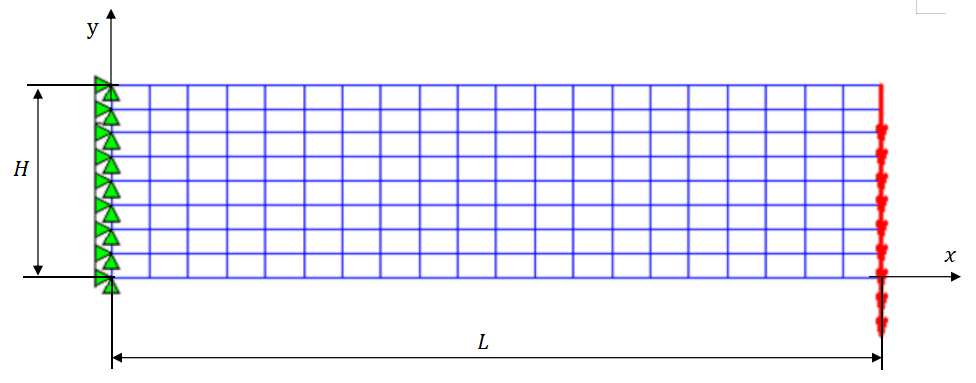
MATLAB example The cantilever has length L = 200 m m L=200\ \mathrm{mm} L = 200 mm H = 50 m m H=50\ \mathrm{mm} H = 50 mm h = 5 m m h=5\ \mathrm{mm} h = 5 mm E = 2.1 × 10 5 M P a E=2.1\times10^5\ \mathrm{MPa} E = 2.1 × 1 0 5 MPa ν = 0.3 \nu=0.3 ν = 0.3 x = 0 x=0 x = 0 u = v = 0 u=v=0 u = v = 0 F = 1000 N F=1000\ \mathrm{N} F = 1000 N x = L x=L x = L
Figure 2. Cantilever geometry, constraints, structured quadrilateral mesh, and uniformly distributed free-end force.The MATLAB program is organized as follows:
gen generates the cantilever mesh, boundary conditions, loads, material data, and model plot.plane2d forms all element stiffness matrices, assembles the global system, imposes the boundary conditions and loads, and solves for the nodal displacements.plot_disp plots the horizontal or vertical displacement map.plot_stress plots the selected stress map.The stiffness routine preserves the explicit Jacobian operations used in the derivation:
J=H*[xel yel];
detJ=abs(det(J));
J1=inv(J);
b=J1*H;
The results are obtained with 40 quadrilateral elements along the beam and 16 elements through its height: 640 finite elements, 697 nodes, and 1394 equations.
Execution status The complete program was executed in MATLAB R2026a. The mesh counts and all reported displacement and stress extrema were reproduced.
08
Displacement results Figure 3. Horizontal displacement u u u Figure 4. Vertical displacement v v v u min = − 0.04574 × 10 − 2 m m , u max = 0.04574 × 10 − 2 m m
u_{\min}=-0.04574\times10^{-2}\ \mathrm{mm},\qquad
u_{\max}=0.04574\times10^{-2}\ \mathrm{mm}
u m i n = − 0.04574 × 1 0 − 2 mm , u m a x = 0.04574 × 1 0 − 2 mm v min = − 0.2535 m m , v max = 0
v_{\min}=-0.2535\ \mathrm{mm},\qquad v_{\max}=0
v m i n = − 0.2535 mm , v m a x = 0 For comparison, the magnitude of the free-end displacement predicted by the Timoshenko beam model is:
∣ v max ∣ T i m o s h e n k o = F L 3 3 E I + 1.2 F L G A = 0.2557 m m
\left|v_{\max}\right|_{\mathrm{Timoshenko}}
=\frac{FL^3}{3EI}+1.2\frac{FL}{GA}
=0.2557\ \mathrm{mm}
∣ v m a x ∣ Timoshenko = 3 E I F L 3 + 1.2 G A F L = 0.2557 mm The finite element displacement is negative because the applied force acts in the negative vertical direction.
09
Stress results For plotting, stresses are evaluated at the element nodes and averaged at nodes shared by adjacent elements.
Figure 5. Normal stress σ x \sigma_x σ x Figure 6. Von Mises stress σ V M \sigma_{\mathrm{VM}} σ VM σ x , min ≈ − 115.22 M P a , σ x , max ≈ 115.22 M P a
\sigma_{x,\min}\approx-115.22\ \mathrm{MPa},\qquad
\sigma_{x,\max}\approx115.22\ \mathrm{MPa}
σ x , m i n ≈ − 115.22 MPa , σ x , m a x ≈ 115.22 MPa σ V M , min ≈ 4.442 M P a , σ V M , max ≈ 109.17 M P a
\sigma_{\mathrm{VM},\min}\approx4.442\ \mathrm{MPa},\qquad
\sigma_{\mathrm{VM},\max}\approx109.17\ \mathrm{MPa}
σ VM , m i n ≈ 4.442 MPa , σ VM , m a x ≈ 109.17 MPa Figure 7. Shear stress τ x y \tau_{xy} τ x y For the rectangular cross-section, the Jourawski formula gives:
τ max = 3 2 V A = 1.5 1000 50 ⋅ 5 = 6 M P a \tau_{\max}=\frac{3}{2}\frac{V}{A}
=1.5\frac{1000}{50\cdot5}
=6\ \mathrm{MPa} τ m a x = 2 3 A V = 1.5 50 ⋅ 5 1000 = 6 MPa At the node located at the center of the rectangular beam domain, the Q4 solution gives ∣ τ x y ∣ = 5.9199 M P a |\tau_{xy}|=5.9199\ \mathrm{MPa} ∣ τ x y ∣ = 5.9199 MPa 6 M P a 6\ \mathrm{MPa} 6 MPa 1.34 % 1.34\% 1.34%
The MATLAB results agree with those obtained with the accompanying ANSYS model.
10
Programs and downloads The MATLAB package was executed in MATLAB R2026a. The ANSYS macro was inspected for consistency with the same geometry, thickness, material, plane-stress model, loading, constraints, and mesh, but was not executed during preparation of this page.
11
Reference C. A. Felippa, Introduction to Finite Element Methods , University of Colorado Boulder, course notes and syllabus. PREVIOUS SECTION ← 9.3. CST: Fast MATLAB Solver — Alternative Version NEXT SECTION 9.5. Isoparametric 4-Node Quadrilateral: Fast Solver →