01
Purpose and benchmark model
plane2d_fast is the vectorized alternative to the standard plane2d routine presented in Section 9.4. It follows the same general strategy as the CST fast solver in Section 9.2: simultaneous element computations with multiprod and direct sparse assembly with MATLAB sparse.
The benchmark uses the plane-stress cantilever of Section 9.4. The mesh has Q4 elements through the height and elements along the length, so that
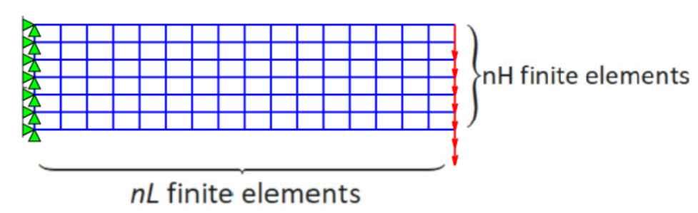
02
Four Gauss-point contributions
Each Q4 finite element is integrated with four Gauss points. The number of vectorized integration contributions is therefore:
The strain-displacement and constitutive matrices are stored for every Gauss-point contribution in three-dimensional arrays:
Thus, the four terms belonging to each finite element are evaluated vectorially. During sparse assembly, their entries have the same element connectivity and are naturally summed at the corresponding global matrix positions.
03
Vectorized element computation
The nodal coordinate arrays are first repeated for the four Gauss points of every element. The Jacobian matrices, their inverses, and the derivatives with respect to the Cartesian coordinates are then evaluated simultaneously for all contributions.
The Q4 strain-displacement matrix has eight columns. Its public implementation therefore uses the explicit preallocation
B=zeros(3,8,nel4);The constitutive matrices include the Gauss-point Jacobian determinant and the element thickness. The simultaneous matrix products are
DB=multiprod(DHooke,B);
kelt=reshape(multiprod(permute(B,[2 1 3]),DB),ngel^2,nel4);
Here DB stores the products for all Gauss points, while each column of kelt contains the 64 entries of one Gauss-point stiffness contribution.
04
Sparse global assembly
The connectivity arrays are expanded to the four Gauss-point contributions. MATLAB sparse then assembles the global stiffness matrix directly and sums coincident entries:
K=sparse(ipos1,ipos2(:),kelt(:),neq,neq);This avoids the element-by-element stiffness-assembly loop. After applying the constraints and loads, the global linear system is solved in the standard form
S=K\F;05
Use with Section 9.4
Start from the complete MATLAB programs provided in Section 9.4, add plane2d_fast.m and multiprod.m, and replace the call plane2d in main.m with plane2d_fast. The geometry, material, loading, constraints, and result-plotting routines remain unchanged.
06
MATLAB R2026a benchmark
For each mesh, both routines received one unrecorded warm-up run followed by three measured runs. The table reports arithmetic means obtained on an Intel Core i7-14700 @ 2.10 GHz computer with 32 GB RAM, Windows 11, and MATLAB 26.1.0 (R2026a) Update 4.
The assembly interval includes element-matrix generation, loads, constraints, and global stiffness assembly. The linear solution was measured separately. Total time is the sum of these two directly measured intervals.
| Q4 elements | Equations | Standardtotal (s) | Fasttotal (s) | Fast K\F(s) | Overallspeed-up | Standardassembly (s) | Fastassembly (s) | Assemblyspeed-up | |
|---|---|---|---|---|---|---|---|---|---|
| 80 × 200 | 16,000 | 32,562 | 19.242 | 0.365 | 0.191 | 52.7× | 19.036 | 0.174 | 109.3× |
| 100 × 250 | 25,000 | 50,702 | 53.805 | 0.508 | 0.282 | 105.9× | 53.518 | 0.227 | 236.1× |
The vectorized Gauss-point calculations and direct sparse assembly reduce the pre-solve interval by more than two orders of magnitude for these meshes. The overall acceleration is smaller because the sparse linear-system solution is essentially the same operation in both implementations.
07
Numerical equivalence
The nodal displacement vectors and recovered element-node stresses were compared before accepting the timings.
| Maximum displacement difference | Relative displacement difference | Maximum stress difference | Relative stress difference | |
|---|---|---|---|---|
| 80 × 200 | ||||
| 100 × 250 |
The differences are consistent with floating-point round-off caused by the different operation ordering.
08
Large-mesh comparison
For a much larger mesh with and , corresponding to 1,253,502 global equations, plane2d_fast required 10.251 s for generation and assembly and 21.082 s for the solution of the global system.
| Fast formulation | Assembly(s) | K\F(s) |
|---|---|---|
| Section 9.2 — CST | 2.553 | 21.487 |
| Section 9.5 — Q4 | 10.251 | 21.082 |
For the same number of global equations, the 4-node quadrilateral formulation requires a longer generation-and-assembly time than the CST formulation because each Q4 element contributes an stiffness matrix rather than a matrix. This produces more nonzero couplings and therefore a denser global stiffness matrix. The Q4 generation-and-assembly interval is approximately times longer, while the linear-system solution times for this case are of the same order.
09
Programs and downloads
The standard and fast Q4 solvers were executed in MATLAB R2026a on both published benchmark meshes. The package contains only the fast routine, multiprod, its BSD license, and a README.
multiprod.m is by Paolo de Leva and is redistributed under the included BSD-style license. Its authoritative distribution page is the MATLAB Central File Exchange entry.