01
Formulation and updating procedures
The isoparametric 4-node quadrilateral finite element is briefly described in Section 9.4.
Updated Lagrangian (UL) formulation. The equations are written with respect to a known current configuration. Two updating procedures are considered. In Section 15.1, the geometry is updated after each iteration, so the Jacobian and spatial derivatives are recomputed using the latest trial configuration. In Section 15.2, the converged configuration of the preceding load step is used throughout the next load step and the geometry is updated only after convergence.
In this section, at each iteration, the nodal coordinates represent the latest known current trial configuration. The routine stiff recomputes the Jacobian, spatial derivatives, and strain–displacement matrices using these coordinates. After the displacement correction is obtained, the coordinates are updated and this new geometry is used in the next iteration. Thus, the derivatives entering the Euler–Almansi relations are evaluated with respect to the latest current trial geometry.
| Total Lagrangian (TL) | Updated Lagrangian (UL) — version 1 Section 15.1 geometry updated after each iteration | Updated Lagrangian (UL) — version 2 Section 15.2 geometry updated after each load step |
|---|---|---|
| The initial configuration is the reference configuration. | The latest current trial configuration is used to recompute geometry-dependent quantities during the iteration. | The converged configuration of the preceding load step remains the reference throughout the next load step. |
| Target quantities are referred to the initial configuration. Derivatives and integrals are evaluated with respect to it. | Target increments are evaluated from the latest trial geometry. Derivatives and integrals use the current trial configuration. | Target increments are referred to the preceding converged configuration. Derivatives and integrals use that configuration. |
| Second Piola–Kirchhoff stress and Green–Lagrange strain | Cauchy stress and Euler–Almansi strain | Cauchy stress and Euler–Almansi strain |
The comparison follows the reference-configuration discussion of Chatzi [1]. For small strains, Green–Lagrange and Euler–Almansi strains become close to their linearized counterparts. Similarly, PK2 and Cauchy stresses have close numerical values when compared in corresponding material and spatial directions. Large rotations may still produce different tensor components when they are expressed in a fixed global coordinate system.
02
Approximate deformation energy
For the present small-strain formulation, the following approximate deformation-energy expression written in the current configuration is used:
In the natural coordinates :
Here, is the known accumulated strain at the beginning of the current load step, is the strain increment produced during the current step, and is the Cauchy stress evaluated at the current iteration. Engineering notation is used:
For a linear elastic plane-stress material:
03
Current geometry and Jacobian
At iteration , the Jacobian is recomputed from the latest trial nodal coordinates:
The current spatial derivatives of the shape functions are obtained from:
The four displacement-gradient relations are:
04
Euler–Almansi strain increments
The explicit two-dimensional Euler–Almansi strain increments are:
The minus signs distinguish these current-configuration increments from the Green–Lagrange expressions used in the Total Lagrangian formulation. Substitution of the displacement interpolation gives:
The symmetric matrices are:
05
Strain–displacement matrix
The strain variation is related to the element nodal displacement variation by:
For the Euler–Almansi component relations:
The negative nonlinear contribution is intentional. If the intermediate variation is written explicitly, the consistent sign is:
06
MATLAB implementation
The Section 12.2 Total Lagrangian program is adapted to update the geometry after every iteration. The three displacement quantities in main have distinct roles:
dSis the displacement correction obtained in one iteration.Sis the displacement increment accumulated during the current load step.St(:,istep+1)is the total accumulated displacement up to the converged load step.
S=zeros(neq,1);
while (error > tol) & (iter < itermax)
    iter=iter+1;
    stiff
    dS=K\F;
    S=S-dS;
    error=sqrt(dS'*dS/neq);
    x=x-dS(1:2:neq);
    y=y-dS(2:2:neq);
end
St(:,istep+1)=St(:,istep)+S;
The geometry update changes after each correction; consequently, stiff uses the latest current trial configuration at the next iteration. Its essential Euler–Almansi and assembly statements are:
% Euler-Almansi strains:
ex =ux-ux^2/2-vx^2/2;
ey =vy-uy^2/2-vy^2/2;
exy=uy+vx-ux*uy-vx*vy;

B=B0-BL;
ex =ex +strnt(ig,1,istep);
ey =ey +strnt(ig,2,istep);
exy=exy+strnt(ig,3,istep);
sigmt(ig,1:3,istep+1)=[ex ey exy]*DHooke;
th1=(1-nu/(1-nu)*(ex+ey))*th;
fel=fel+th1*(B'*sigmt(ig,1:3,istep+1)')*detJ;
kel=kel+th1*(B'*DHooke*B)*detJ;
In theoretical notation, these element vectors and matrices are assembled into the global quantities as:
Here, denotes the standard finite-element assembly operator, which places the element contributions into the corresponding global degrees of freedom and adds overlapping contributions.
For a plane-stress state and small strains, the thickness strain is approximated by:
Therefore, the current thickness used by the program is:
This thickness relation is a small-strain approximation; it is not a general exact relation for finite elastic strains.
The stresses are known at the four Gauss points. For each element, plot_stress fits the linear plane:
The existing least-squares equations determine the coefficients from the Gauss-point stresses. The fitted plane is evaluated at the four element nodes, and contributions from elements sharing a node are averaged arithmetically. The strain plotting routine uses the same extrapolation and averaging structure for strains.
07
Simplified tangent and incremental approximation
A simplified tangent stiffness is used in the present UL implementation. Since the geometry is updated after every iteration, the Jacobian and the strain–displacement matrices are recomputed for the latest current configuration. The geometric terms used in the TL tangent stiffness are therefore not transferred directly to the present formulation. Numerical tests showed that introducing these TL-type terms deteriorated convergence, whereas the simplified tangent used here produced a stable iterative process. This matrix is an approximate tangent stiffness; a fully consistent UL tangent would require a separate linearization in the current configuration.
Within the adopted UL model, the internal-force vector is evaluated directly from the current trial state, whereas the tangent stiffness used for the iterative correction is deliberately simplified. Thus, the additional approximation introduced in the tangent stiffness does not alter the direct evaluation of the internal-force vector at each iteration.
For one finite element, the implemented approximation is:
The internal-force vector is recalculated at every iteration from the current geometry and stresses:
The present formulation uses an approximate incremental update. At each iteration, the equations are evaluated using the latest known geometry, which is subsequently updated by the newly calculated displacement correction. Euler–Almansi strain increments are accumulated over successive load steps. For small strains and sufficiently small load increments, the discrepancies introduced by these approximations become small and decrease as the load-step size is reduced.
08
Example 1: axial tension
A cantilever-like prismatic bar has initial length , rectangular cross-section , Young’s modulus , Poisson ratio , and an axial force applied at its free end.
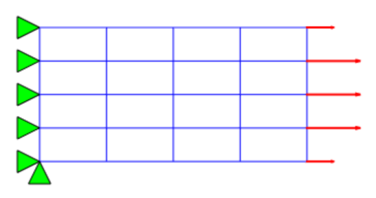
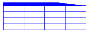
For the present one-dimensional model, Poisson contraction gives the current area . The analytical Cauchy stress is:
Using , the strain is obtained from the cubic equation:
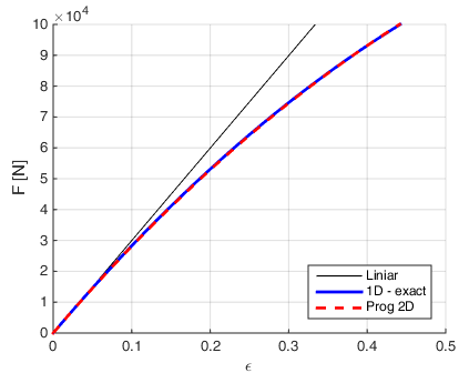
The unusually large strain range is used only to emphasize the trend of the curves. It lies outside the strict small-strain range assumed by the formulation and should therefore be regarded as a numerical illustration rather than as a finite-strain constitutive validation.
The one-dimensional Euler–Almansi relation itself gives directly:
Therefore:
The recursive development is nevertheless retained because it reproduces the incremental updating used by the UL finite-element algorithm. For , the cubic equation is solved at each interval:
For a sufficiently small increment:
The recursive formula is:
clear
E=1000;   % Young's modulus
nu=0.3;   % Poisson ratio
A=300;    % cross-section area
L0=100;   % initial length
F0=80000; % force
nf=5000;  % number of points
dF=F0/nf;
uu(1)=0;
for i=1:nf
    FF(i+1,1)=i*F0/nf;
    p=[nu^2 -2*nu 1 -FF(i+1)/E/A];
    eer=roots(p);
    ee(i+1,1)=eer(3);
    uu(i+1)=uu(i)+(ee(i+1)-ee(i))*(L0+uu(i));
end
figure(1), clf, hold on, grid on
plot([0 max(ee)],[0 max(ee)*L0],'k')
plot(ee,uu,'r','linewidth',1.5)
xlabel('\epsilon')
ylabel('u [mm]')
legend('Linear','1D analytical','Location','southeast')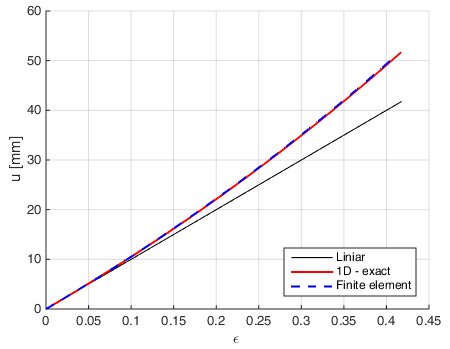
09
Example 2: cantilever comparison
The cantilever beam has length and a rectangular cross-section . The material properties are and . A vertical force is applied at the free end. The mesh contains Q4 elements and 2,057 nodes. The load is applied in 50 load steps.
The displacement results show very good agreement among TL, UL, and ANSYS. Stress components require a more careful comparison: TL reports second Piola–Kirchhoff stress, whereas UL and ANSYS report Cauchy stress. In addition, strains near the clamped end reach approximately , which is outside the strict small-strain range assumed by the formulation. Large rotations and the different configurations in which the stress tensors are expressed also influence comparisons of global components.
The MATLAB R2026a run completed all 50 load steps, with no more than 6 iterations per step. At the final step, the calculated extrema were , , , , and .
10
Programs and downloads
11
References
Eleni Chatzi, The Finite Element Method for the Analysis of Non-Linear and Dynamic Systems, ETH Zürich, Lecture 3, 15 October 2015.