23.4. Differential equilibrium equations for 3D slender curved beams

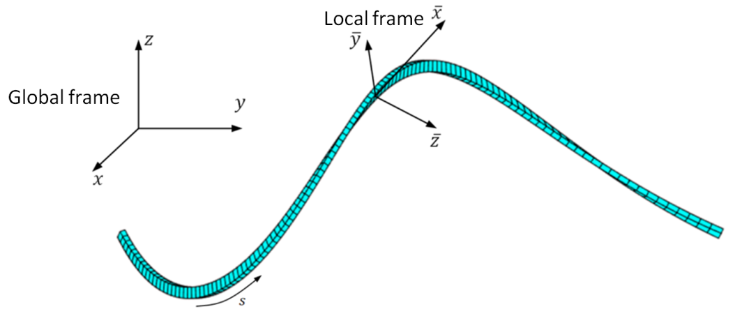
A 3D slender curved beam may be regarded as generated by a cross-section moving along a three-dimensional curved centroidal axis while remaining normal to it. The centroid of each cross-section lies on this curve, and the dimensions of the cross-section are small compared with the other dimensions of the beam.

At every point of the centroidal axis, the rotation matrix $\boldsymbol{R}$ is known as a function of the curvilinear coordinate $s$ . As in Section 22.1, $\boldsymbol{R}$ is the passive transformation matrix from the global reference frame to the local reference frame:

\bar{\boldsymbol{v}}=\boldsymbol{R}\boldsymbol{v} .

Thus, $\boldsymbol{R}(s)$ defines the local reference frame

\bar{\mathcal X}=(\bar x,\bar y,\bar z)

of each cross-section with respect to the global reference frame

\mathcal X=(x,y,z).

The $\bar x$ -axis is tangent to the centroidal axis, while the $\bar y$ - and $\bar z$ -axes coincide with the two central principal axes of the cross-section. Therefore, the geometry of the beam is completely characterised when the cross-section and the matrix $\boldsymbol{R}(s)$ are known.

**Figure 1.** Curved beam and reference frames.

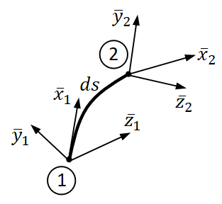
Let us consider two neighbouring cross-sections, ① and ②, separated by the infinitesimal distance $ds$ . Their relative rotation is infinitesimal and may therefore be represented by the vector

d\boldsymbol{\varphi} = \begin{Bmatrix} d\varphi_{\bar x}\\ d\varphi_{\bar y}\\ d\varphi_{\bar z} \end{Bmatrix}.

The curvature components are defined as

\kappa_{\bar x}=\frac{d\varphi_{\bar x}}{ds}, \qquad \kappa_{\bar y}=\frac{d\varphi_{\bar y}}{ds}, \qquad \kappa_{\bar z}=\frac{d\varphi_{\bar z}}{ds}.

For two infinitesimally close cross-sections, the relative rotation matrix is

\boldsymbol{R}_0= \begin{bmatrix} 1 & -d\varphi_{\bar z} & d\varphi_{\bar y}\\ d\varphi_{\bar z} & 1 & -d\varphi_{\bar x}\\ -d\varphi_{\bar y} & d\varphi_{\bar x} & 1 \end{bmatrix}.

If cross-section ① is characterised by $\boldsymbol{R}$ , cross-section ② is characterised by $\boldsymbol{R}_0\boldsymbol{R}$ . Hence,

\frac{d\boldsymbol{R}}{ds} = \frac{1}{ds}(\boldsymbol{R}_0\boldsymbol{R}-\boldsymbol{R}) = \frac{1}{ds}(\boldsymbol{R}_0-\boldsymbol{I})\boldsymbol{R} = \tilde{\boldsymbol{\kappa}}\boldsymbol{R} ,

where

\boxed{ \tilde{\boldsymbol{\kappa}} = \frac{d\boldsymbol{R}}{ds}\boldsymbol{R}^T }

is the skew-symmetric curvature tensor:

\tilde{\boldsymbol{\kappa}} = \begin{bmatrix} 0 & -\kappa_{\bar z} & \kappa_{\bar y}\\ \kappa_{\bar z} & 0 & -\kappa_{\bar x}\\ -\kappa_{\bar y} & \kappa_{\bar x} & 0 \end{bmatrix}.

The curvature components may also be collected in the vector:

\boldsymbol{\kappa} = \begin{Bmatrix} \kappa_{\bar x}\\ \kappa_{\bar y}\\ \kappa_{\bar z} \end{Bmatrix}.

On each cross-section act six internal resultants: the axial force $N$ , the two shear forces $T_{\bar y}$ and $T_{\bar z}$ , the torque $M_{\bar x}$ , and the two bending moments $M_{\bar y}$ and $M_{\bar z}$ .

They are conveniently grouped into the local force and moment vectors:

\bar{\boldsymbol{F}} = \begin{Bmatrix} N\\ T_{\bar y}\\ T_{\bar z} \end{Bmatrix}, \qquad \bar{\boldsymbol{M}} = \begin{Bmatrix} M_{\bar x}\\ M_{\bar y}\\ M_{\bar z} \end{Bmatrix}.

The corresponding vectors in the global reference frame are

\boldsymbol{F}= \begin{Bmatrix} F_x\\ F_y\\ F_z \end{Bmatrix}, \qquad \boldsymbol{M}= \begin{Bmatrix} M_x\\ M_y\\ M_z \end{Bmatrix},

and, according to the adopted passive transformation,

\boxed{ \bar{\boldsymbol{F}}=\boldsymbol{R}\boldsymbol{F}, \qquad \bar{\boldsymbol{M}}=\boldsymbol{R}\boldsymbol{M}. }

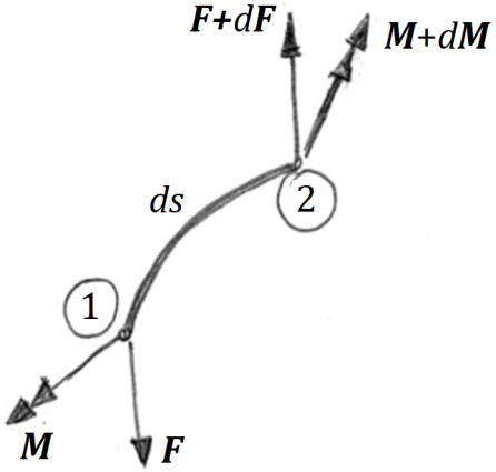
Consider now an infinitesimal beam element of length $ds$ . Let $\boldsymbol{q}$ denote the distributed force per unit length, expressed in the global reference frame, and let

\bar{\boldsymbol{q}}=\boldsymbol{R}\boldsymbol{q}

be the corresponding local vector.

**Figure 3.** Internal resultants on an infinitesimal beam element.

Let $\boldsymbol{t}$ be the unit tangent to the centroidal axis, oriented in the direction of increasing $s$ . In the local frame,

\boldsymbol{R}\boldsymbol{t}= \begin{Bmatrix} 1\\ 0\\ 0 \end{Bmatrix}.

The differential equilibrium equations written in the global reference frame are

\frac{d\boldsymbol{F}}{ds}=-\boldsymbol{q}

and

\frac{d\boldsymbol{M}}{ds} = -\boldsymbol{t}\times\boldsymbol{F}.

Differentiating the local force vector,

\frac{d\bar{\boldsymbol{F}}}{ds} = \frac{d}{ds}(\boldsymbol{R}\boldsymbol{F}) = \frac{d\boldsymbol{R}}{ds}\boldsymbol{F} + \boldsymbol{R}\frac{d\boldsymbol{F}}{ds},

and using

\frac{d\boldsymbol{R}}{ds} = \tilde{\boldsymbol{\kappa}}\boldsymbol{R},

we obtain

\boxed{ \frac{d\bar{\boldsymbol{F}}}{ds} = \tilde{\boldsymbol{\kappa}}\bar{\boldsymbol{F}} - \bar{\boldsymbol{q}}. }

Similarly,

\frac{d\bar{\boldsymbol{M}}}{ds} = \frac{d}{ds}(\boldsymbol{R}\boldsymbol{M}) = \tilde{\boldsymbol{\kappa}}\bar{\boldsymbol{M}} + \boldsymbol{R}\frac{d\boldsymbol{M}}{ds}.

Since rotations preserve the cross product,

\boldsymbol{R}(\boldsymbol{t}\times\boldsymbol{F}) = (\boldsymbol{R}\boldsymbol{t})\times(\boldsymbol{R}\boldsymbol{F}),

and therefore

- \begin{Bmatrix} 1\\ 0\\ 0 \end{Bmatrix} \times \begin{Bmatrix} N\\ T_{\bar y}\\ T_{\bar z} \end{Bmatrix} = \begin{Bmatrix} 0\\ T_{\bar z}\\ -T_{\bar y} \end{Bmatrix}.

Finally,

\boxed{ \frac{d\bar{\boldsymbol{M}}}{ds} = \tilde{\boldsymbol{\kappa}}\bar{\boldsymbol{M}} + \begin{Bmatrix} 0\\ T_{\bar z}\\ -T_{\bar y} \end{Bmatrix}. }

These two vector equations are the differential equilibrium equations of a 3D slender curved beam.

For a 2D curved beam lying in the $(\bar x,\bar y)$ plane,

\kappa_{\bar x}=0, \qquad \kappa_{\bar y}=0, \qquad \kappa_{\bar z}=\frac{1}{r},

and the equilibrium equations reduce to

\frac{dN}{ds} = -\frac{T_{\bar y}}{r} - q_{\bar x},

\frac{dT_{\bar y}}{ds} = \frac{N}{r} - q_{\bar y},

\frac{dM_{\bar z}}{ds} = -T_{\bar y}.

For a straight beam,

\kappa_{\bar x} = \kappa_{\bar y} = \kappa_{\bar z} = 0,

and the well-known differential equilibrium equations are recovered:

\frac{dN}{dx}=-q_x, \qquad \frac{dT_y}{dx}=-q_y, \qquad \frac{dM_z}{dx}=-T_y.

The differential equilibrium equations derived above are generally valid. In the case of 3D beams undergoing large displacements, they must be formulated in the current deformed configuration.

Example

Let us consider an initially straight cantilever beam of length

L=100\ {\rm mm},

located along the global $x$ -axis and clamped at the node situated at the origin. The beam has a rectangular cross-section $2.5\ {\rm mm}\times3.5\ {\rm mm}$ (width $\times$ thickness) and Young's modulus

E=2\times10^5\ {\rm MPa}.

The following forces and moments are applied at the free end:

X=-300\ {\rm N}, \qquad Y=100\ {\rm N}, \qquad Z=50\ {\rm N},

C_x=30\,000\ {\rm Nmm}, \qquad C_y=0, \qquad C_z=40\,000\ {\rm Nmm}.

The deformed configuration is obtained with the large-displacement 3D cantilever program presented in Section 22.2.

Figure 4. Deformed configuration of the cantilever beam.

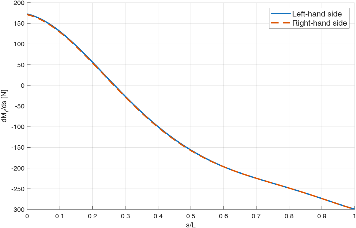
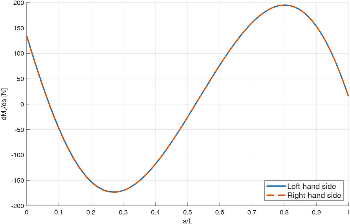
For this deformed configuration, the two sides of the moment-equilibrium equation

\boxed{ \frac{d\bar{\boldsymbol{M}}}{ds} = \tilde{\boldsymbol{\kappa}}\bar{\boldsymbol{M}} + \begin{Bmatrix} 0\\ T_{\bar z}\\ -T_{\bar y} \end{Bmatrix} }

are evaluated independently along the beam.

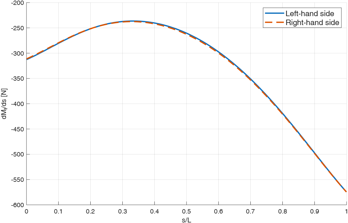
The three components correspond respectively to torsion, bending about the $\bar y$ -axis, and bending about the $\bar z$ -axis. The diagrams below compare the left-hand and right-hand sides of the equilibrium equation.

**Figure 6.** Bending equilibrium about the local y-axis.

**Figure 7.** Bending equilibrium about the local z-axis.

The practically coincident curves confirm the differential moment-equilibrium equations along the deformed beam.

The MATLAB programs used for this example, including the program presented in Section 22.2 with the input data modified for the present case, can be downloaded here as a ZIP archive.

MATLAB3D cantilever — equilibrium verificationDownload ZIP