Chapter 19

Buckling of beam structures

Linear buckling analysis using Euler–Bernoulli and Timoshenko beam finite elements.

Small strainLinear elasticBeam structuresEigenvalue buckling

01

Energy formulation

Small displacements
Small strains
Linear elastic material

Although the displacements are assumed to be small, the second-order terms in the strain–displacement relations are retained because they are essential for the stability analysis. These terms generate the geometric stiffness matrix. [1]

Buckling is a bifurcation phenomenon. The structure follows the small-displacement equilibrium path up to a critical load, at which this equilibrium state loses stability and a new equilibrium path associated with lateral deformation becomes possible. Along the post-buckling path, large displacements may subsequently develop.

The strain energy of a beam element is:

Uel=12LεTDεdxˉU_\mathrm{el}=\frac12\int_L\boldsymbol{\varepsilon}^{T}\boldsymbol{D}\boldsymbol{\varepsilon}\,d\bar x

The following developments retain all the terms required to obtain both the elastic stiffness matrix and the geometric stiffness matrix.

02

Euler–Bernoulli beam model

For the Euler–Bernoulli beam model, the constitutive matrix and the generalized strain vector are:
D=[EA00EI]\boldsymbol{D}=\begin{bmatrix}EA&0\\0&EI\end{bmatrix}
ε={ε0κ}={duˉ/dxˉd2vˉ/dxˉ2}={uˉvˉ}\boldsymbol{\varepsilon}=\left\{\begin{array}{c}\varepsilon_0\\\kappa\end{array}\right\}=\left\{\begin{array}{c}d\bar u/d\bar x\\d^2\bar v/d\bar x^2\end{array}\right\}=\left\{\begin{array}{c}\bar u'\\\bar v''\end{array}\right\}
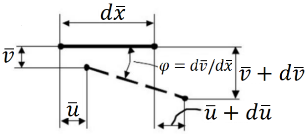
Deformation of an Euler–Bernoulli beam element
Figure 1. Deformation and kinematic quantities of a beam element.

When the second-order contribution produced by the transverse displacement is retained, the axial strain contains the additional term (see Chapter 6):

ε={uˉ+12vˉ2vˉ}={ε0+12vˉ2κ}.\boxed{\boldsymbol{\varepsilon}=\left\{\begin{array}{c}\bar u'+\frac12\bar v'^2\\\bar v''\end{array}\right\}=\left\{\begin{array}{c}\varepsilon_0+\frac12\bar v'^2\\\kappa\end{array}\right\}.}

After substitution in the strain energy and neglecting terms of order higher than two, the expression can be separated into an elastic part and a part that depends on the axial force:

Uel=12L[EA(uˉ)2+EI(vˉ)2+N(vˉ)2]dxˉ,N=EAε0U_{\rm el}=\frac12\int_L\left[EA(\bar u')^2+EI(\bar v'')^2+N(\bar v')^2\right]d\bar x,\qquad N=EA\,\varepsilon_0

The generalized strains and the slope of the beam axis are written as:

{ε0κ}=Buel,φ=dvˉdxˉ=Nφuel\left\{\begin{array}{c}\varepsilon_0\\\kappa\end{array}\right\}=\boldsymbol{B}\boldsymbol{u}_{\rm el},\qquad \varphi=\frac{d\bar v}{d\bar x}=\boldsymbol{N}_{\varphi}\boldsymbol{u}_{\rm el}
uel={uˉ1vˉ1φ1uˉ2vˉ2φ2}T\boldsymbol{u}_{\rm el}=\left\{\begin{array}{cccccc}\bar u_1&\bar v_1&\varphi_1&\bar u_2&\bar v_2&\varphi_2\end{array}\right\}^{T}

With ξ=xˉ/L\xi=\bar x/L, the displacement interpolation matrix is:

{uˉvˉφ}=[1ξ00ξ0002ξ33ξ2+1(ξ32ξ2+ξ)L02ξ3+3ξ2(ξ3ξ2)L0(6ξ26ξ)/L3ξ24ξ+10(6ξ2+6ξ)/L3ξ22ξ]uel\left\{\begin{array}{c}\bar u\\\bar v\\\varphi\end{array}\right\}=\begin{bmatrix}1-\xi&0&0&\xi&0&0\\0&2\xi^3-3\xi^2+1&(\xi^3-2\xi^2+\xi)L&0&-2\xi^3+3\xi^2&(\xi^3-\xi^2)L\\0&(6\xi^2-6\xi)/L&3\xi^2-4\xi+1&0&(-6\xi^2+6\xi)/L&3\xi^2-2\xi\end{bmatrix}\boldsymbol{u}_{\rm el}
B=[1/L001/L000(12ξ6)/L2(6ξ4)/L0(12ξ+6)/L2(6ξ2)/L]\boldsymbol{B}=\begin{bmatrix}-1/L&0&0&1/L&0&0\\0&(12\xi-6)/L^2&(6\xi-4)/L&0&(-12\xi+6)/L^2&(6\xi-2)/L\end{bmatrix}
Nφ=[0(6ξ26ξ)/L3ξ24ξ+10(6ξ2+6ξ)/L3ξ22ξ]\boldsymbol{N}_{\varphi}=\begin{bmatrix}0&(6\xi^2-6\xi)/L&3\xi^2-4\xi+1&0&(-6\xi^2+6\xi)/L&3\xi^2-2\xi\end{bmatrix}

The element strain energy becomes:

Uel=12uelTkeluel=12uelT(k0+kG)uelU_{\rm el}=\frac12\boldsymbol{u}_{\rm el}^{T}\boldsymbol{k}_{\rm el}\boldsymbol{u}_{\rm el}=\frac12\boldsymbol{u}_{\rm el}^{T}(\boldsymbol{k}_0+\boldsymbol{k}_G)\boldsymbol{u}_{\rm el}
k0=LBTDBdxˉ,kG=NLNφTNφdxˉ\boldsymbol{k}_0=\int_L\boldsymbol{B}^{T}\boldsymbol{D}\boldsymbol{B}\,d\bar x,\qquad \boxed{\boldsymbol{k}_G=-N\int_L\boldsymbol{N}_{\varphi}^{T}\boldsymbol{N}_{\varphi}\,d\bar x}

For the two-node Euler–Bernoulli element, integration gives:

k0=[EA/L00EA/L00012EI/L36EI/L2012EI/L36EI/L206EI/L24EI/L06EI/L22EI/LEA/L00EA/L00012EI/L36EI/L2012EI/L36EI/L206EI/L22EI/L06EI/L24EI/L]\boldsymbol{k}_0=\begin{bmatrix}EA/L&0&0&-EA/L&0&0\\0&12EI/L^3&6EI/L^2&0&-12EI/L^3&6EI/L^2\\0&6EI/L^2&4EI/L&0&-6EI/L^2&2EI/L\\-EA/L&0&0&EA/L&0&0\\0&-12EI/L^3&-6EI/L^2&0&12EI/L^3&-6EI/L^2\\0&6EI/L^2&2EI/L&0&-6EI/L^2&4EI/L\end{bmatrix}
kG=NL[00000006/5L/1006/5L/100L/102L2/150L/10L2/3000000006/5L/1006/5L/100L/10L2/300L/102L2/15]\boldsymbol{k}_G=\frac{-N}{L}\begin{bmatrix}0&0&0&0&0&0\\0&6/5&L/10&0&-6/5&L/10\\0&L/10&2L^2/15&0&-L/10&-L^2/30\\0&0&0&0&0&0\\0&-6/5&-L/10&0&6/5&-L/10\\0&L/10&-L^2/30&0&-L/10&2L^2/15\end{bmatrix}

03

Timoshenko beam model — isoparametric linear element

The Timoshenko beam model includes shear deformation. The axial strain, shear strain and curvature are:

ε={ε0βκ}+{12(vˉ)200},D=[EA000GA0000EI]\boldsymbol{\varepsilon}=\left\{\begin{array}{c}\varepsilon_0\\\beta\\\kappa\end{array}\right\}+\left\{\begin{array}{c}\frac12(\bar v')^2\\0\\0\end{array}\right\},\qquad \boldsymbol{D}=\begin{bmatrix}EA&0&0\\0&GA_0&0\\0&0&EI\end{bmatrix}
{ε0βκ}={duˉ/dxˉdvˉ/dxˉψdψ/dxˉ}=Buel\left\{\begin{array}{c}\varepsilon_0\\\beta\\\kappa\end{array}\right\}=\left\{\begin{array}{c}d\bar u/d\bar x\\d\bar v/d\bar x-\psi\\d\psi/d\bar x\end{array}\right\}=\boldsymbol{B}\boldsymbol{u}_{\rm el}

The linear isoparametric shape functions are:

h1(s)=1s2,h2(s)=1+s2,s[1,1]h_1(s)=\frac{1-s}{2},\qquad h_2(s)=\frac{1+s}{2},\qquad s\in[-1,1]
uˉ=h1uˉ1+h2uˉ2,vˉ=h1vˉ1+h2vˉ2,ψ=h1ψ1+h2ψ2\bar u=h_1\bar u_1+h_2\bar u_2,\qquad \bar v=h_1\bar v_1+h_2\bar v_2,\qquad \psi=h_1\psi_1+h_2\psi_2
B=[1/L001/L0001/Lh101/Lh2001/L001/L]\boldsymbol{B}=\begin{bmatrix}-1/L&0&0&1/L&0&0\\0&-1/L&-h_1&0&1/L&-h_2\\0&0&-1/L&0&0&1/L\end{bmatrix}

The slope of the beam axis is:

φ=dvˉdxˉ=vˉ1L+vˉ2L\varphi=\frac{d\bar v}{d\bar x}=-\frac{\bar v_1}{L}+\frac{\bar v_2}{L}
Nφ=[01/L001/L0]\boxed{\boldsymbol{N}_{\varphi}=\begin{bmatrix}0&-1/L&0&0&1/L&0\end{bmatrix}}

Since ds/dxˉ=2/Lds/d\bar x=2/L, the element matrices are:

k0=LBTDBdxˉ,kG=NLNφTNφdxˉ\boldsymbol{k}_0=\int_L\boldsymbol{B}^{T}\boldsymbol{D}\boldsymbol{B}\,d\bar x,\qquad \boldsymbol{k}_G=-N\int_L\boldsymbol{N}_{\varphi}^{T}\boldsymbol{N}_{\varphi}\,d\bar x

With one-point Gauss integration, the elastic stiffness matrix used in the program is:

k0=[EA/L00EA/L000GA0/LGA0/20GA0/LGA0/20GA0/2(GA0L2+4EI)/(4L)0GA0/2(GA0L24EI)/(4L)EA/L00EA/L000GA0/LGA0/20GA0/LGA0/20GA0/2(GA0L24EI)/(4L)0GA0/2(GA0L2+4EI)/(4L)]\boldsymbol{k}_0=\begin{bmatrix}EA/L&0&0&-EA/L&0&0\\0&GA_0/L&GA_0/2&0&-GA_0/L&GA_0/2\\0&GA_0/2&(GA_0L^2+4EI)/(4L)&0&-GA_0/2&(GA_0L^2-4EI)/(4L)\\-EA/L&0&0&EA/L&0&0\\0&-GA_0/L&-GA_0/2&0&GA_0/L&-GA_0/2\\0&GA_0/2&(GA_0L^2-4EI)/(4L)&0&-GA_0/2&(GA_0L^2+4EI)/(4L)\end{bmatrix}
kG=NL{010010}{010010}\boldsymbol{k}_G=\frac{-N}{L}\left\{\begin{array}{c}0\\-1\\0\\0\\1\\0\end{array}\right\}\left\{\begin{array}{cccccc}0&-1&0&0&1&0\end{array}\right\}

04

Timoshenko beam model — third-degree shape function

A third-degree interpolation of the transverse displacement improves the behavior of the Timoshenko element. The axial displacement remains linear, while the transverse displacement and section rotation are interpolated consistently.

uˉ=(1ξ)uˉ1+ξuˉ2,vˉ=N2vˉ1+N3ψ1+N5vˉ2+N6ψ2,ξ=xˉ/L\bar u=(1-\xi)\bar u_1+\xi\bar u_2,\qquad \bar v=N_2\bar v_1+N_3\psi_1+N_5\bar v_2+N_6\psi_2,\qquad \xi=\bar x/L

The slope of the beam axis, φ=dvˉ/dxˉ\varphi=d\bar v/d\bar x (see Section 5.2), is obtained by differentiating this interpolation.

N2=12EI+6GA0L2(ξξ2)L(12EI+GA0L2),N3=EI(612ξ)+GA0L2(14ξ+3ξ2)12EI+GA0L2N_2=-\frac{12EI+6GA_0L^2(\xi-\xi^2)}{L(12EI+GA_0L^2)},\qquad N_3=\frac{EI(6-12\xi)+GA_0L^2(1-4\xi+3\xi^2)}{12EI+GA_0L^2}
N5=12EI+6GA0L2(ξξ2)L(12EI+GA0L2),N6=EI(612ξ)+GA0L2(2ξ3ξ2)12EI+GA0L2N_5=\frac{12EI+6GA_0L^2(\xi-\xi^2)}{L(12EI+GA_0L^2)},\qquad N_6=-\frac{EI(6-12\xi)+GA_0L^2(2\xi-3\xi^2)}{12EI+GA_0L^2}

The generalized strain matrix keeps the form:

B=[1/L001/L00012EI/(GA0L3+12EIL)6EI/(GA0L2+12EI)012EI/(GA0L3+12EIL)6EI/(GA0L2+12EI)06GA0(2ξ1)/(GA0L2+12EI)[GA0(46ξ)L2+12EI]/(GA0L3+12EIL)06GA0(2ξ1)/(GA0L2+12EI)[GA0(6ξ2)L2+12EI]/(GA0L3+12EIL)]\boldsymbol{B}=\begin{bmatrix}-1/L&0&0&1/L&0&0\\0&-12EI/(GA_0L^3+12EIL)&-6EI/(GA_0L^2+12EI)&0&12EI/(GA_0L^3+12EIL)&-6EI/(GA_0L^2+12EI)\\0&6GA_0(2\xi-1)/(GA_0L^2+12EI)&[GA_0(4-6\xi)L^2+12EI]/(GA_0L^3+12EIL)&0&-6GA_0(2\xi-1)/(GA_0L^2+12EI)&[GA_0(6\xi-2)L^2+12EI]/(GA_0L^3+12EIL)\end{bmatrix}

Let's check the above expressions. If GA0GA_0\rightarrow\infty, the Timoshenko beam model becomes the Euler–Bernoulli one. The middle row of B\boldsymbol{B} becomes zero and disappears, as in Chapter 6:

B[1/L001/L000(12ξ+6)/L2(6ξ+4)/L0(12ξ6)/L2(6ξ+2)/L]\boldsymbol{B}\longrightarrow\begin{bmatrix}-1/L&0&0&1/L&0&0\\0&(-12\xi+6)/L^2&(-6\xi+4)/L&0&(12\xi-6)/L^2&(-6\xi+2)/L\end{bmatrix}

The slope matrix also becomes the third row of the interpolation matrix given in Chapter 6:

Nφ[06(ξ2ξ)/L14ξ+3ξ206(ξξ2)/L3ξ22ξ]\boldsymbol{N}_{\varphi}\longrightarrow\begin{bmatrix}0&6(\xi^2-\xi)/L&1-4\xi+3\xi^2&0&6(\xi-\xi^2)/L&3\xi^2-2\xi\end{bmatrix}

The elastic and geometric matrices are again obtained from:

k0=LBTDBdxˉ,kG=NLNφTNφdxˉ\boldsymbol{k}_0=\int_L\boldsymbol{B}^{T}\boldsymbol{D}\boldsymbol{B}\,d\bar x,\qquad \boldsymbol{k}_G=-N\int_L\boldsymbol{N}_{\varphi}^{T}\boldsymbol{N}_{\varphi}\,d\bar x

The elastic stiffness matrix is:

k0=[EAL00EAL0001L312EI+LGA01L26EI+2GA001L312EI+LGA01L26EI+2GA001L26EI+2GA043+4EIGA0L2L3EI+4GA0L01L26EI+2GA0234EIGA0L2L3EI+4GA0LEAL00EAL0001L312EI+LGA01L26EI+2GA001L312EI+LGA01L26EI+2GA001L26EI+2GA0234EIGA0L2L3EI+4GA0L01L26EI+2GA043+4EIGA0L2L3EI+4GA0L]\boldsymbol{k}_0=\begin{bmatrix}\dfrac{EA}{L}&0&0&-\dfrac{EA}{L}&0&0\\0&\dfrac{1}{\dfrac{L^3}{12EI}+\dfrac{L}{GA_0}}&\dfrac{1}{\dfrac{L^2}{6EI}+\dfrac{2}{GA_0}}&0&-\dfrac{1}{\dfrac{L^3}{12EI}+\dfrac{L}{GA_0}}&\dfrac{1}{\dfrac{L^2}{6EI}+\dfrac{2}{GA_0}}\\0&\dfrac{1}{\dfrac{L^2}{6EI}+\dfrac{2}{GA_0}}&\dfrac{\dfrac43+\dfrac{4EI}{GA_0L^2}}{\dfrac{L}{3EI}+\dfrac{4}{GA_0L}}&0&-\dfrac{1}{\dfrac{L^2}{6EI}+\dfrac{2}{GA_0}}&\dfrac{\dfrac23-\dfrac{4EI}{GA_0L^2}}{\dfrac{L}{3EI}+\dfrac{4}{GA_0L}}\\-\dfrac{EA}{L}&0&0&\dfrac{EA}{L}&0&0\\0&-\dfrac{1}{\dfrac{L^3}{12EI}+\dfrac{L}{GA_0}}&-\dfrac{1}{\dfrac{L^2}{6EI}+\dfrac{2}{GA_0}}&0&\dfrac{1}{\dfrac{L^3}{12EI}+\dfrac{L}{GA_0}}&-\dfrac{1}{\dfrac{L^2}{6EI}+\dfrac{2}{GA_0}}\\0&\dfrac{1}{\dfrac{L^2}{6EI}+\dfrac{2}{GA_0}}&\dfrac{\dfrac23-\dfrac{4EI}{GA_0L^2}}{\dfrac{L}{3EI}+\dfrac{4}{GA_0L}}&0&-\dfrac{1}{\dfrac{L^2}{6EI}+\dfrac{2}{GA_0}}&\dfrac{\dfrac43+\dfrac{4EI}{GA_0L^2}}{\dfrac{L}{3EI}+\dfrac{4}{GA_0L}}\end{bmatrix}

For the geometric stiffness matrix, it results:

kG=NL[0000000a2a10a2a10a1a40a1a30000000a2a10a2a10a1a30a1a4]\boldsymbol{k}_G=\frac{-N}{L}\begin{bmatrix}0&0&0&0&0&0\\0&a_2&a_1&0&-a_2&a_1\\0&a_1&a_4&0&-a_1&a_3\\0&0&0&0&0&0\\0&-a_2&-a_1&0&a_2&-a_1\\0&a_1&a_3&0&-a_1&a_4\end{bmatrix}
a1=L4(GA0)210a5,a2=L(1L2+L2(GA0)25a5),a3=L(L4(GA0)220a5112)a_1=\frac{L^4(GA_0)^2}{10a_5},\qquad a_2=L\left(\frac{1}{L^2}+\frac{L^2(GA_0)^2}{5a_5}\right),\qquad a_3=L\left(\frac{L^4(GA_0)^2}{20a_5}-\frac{1}{12}\right)
a4=L(L4(GA0)220a5+112),a5=(GA0L2+12EI)2a_4=L\left(\frac{L^4(GA_0)^2}{20a_5}+\frac{1}{12}\right),\qquad a_5=(GA_0L^2+12EI)^2

The local matrices are transformed to the global coordinate frame:

k0,g=RTk0R,kG,g=RTkGR\boldsymbol{k}_{0,g}=\boldsymbol{R}^{T}\boldsymbol{k}_{0}\boldsymbol{R},\qquad \boldsymbol{k}_{G,g}=\boldsymbol{R}^{T}\boldsymbol{k}_{G}\boldsymbol{R}

05

Buckling eigenvalue problem

The element matrices are assembled into the global elastic and geometric stiffness matrices. After applying the boundary conditions, the buckling problem is:

(KλKG)u=0\boxed{(\boldsymbol{K}-\lambda\boldsymbol{K}_G)\boldsymbol{u}=\boldsymbol{0}}

or, equivalently:

Ku=λKGu\boxed{\boldsymbol{K}\boldsymbol{u}=\lambda\boldsymbol{K}_G\boldsymbol{u}}

With the sign convention used here, the axial force NN is negative in compression. The geometric stiffness matrix of a compressed member is therefore assembled using N-N.

The eigenvalue λ\lambda is a load multiplier applied to the reference loading used in the preliminary linear analysis. Since a unit compressive load is used in the present examples, the numerical value of the smallest positive eigenvalue is equal to the critical buckling load in newtons. For a structure subjected to several loads, the same eigenvalue multiplies the complete prescribed reference loading pattern.

06

MATLAB programs

The main program has a very simple structure:

main.m
% main
clear
gen
stiff
S=K\F;
stress
geomK

The gen subprogram generates the input data. The stiff subprogram generates the global stiffness matrix and applies the boundary conditions. The linear system is then solved. The stress subprogram computes the axial forces in the elements, and geomK generates the geometric stiffness matrix and solves the eigenvalue problem.

The matrices used here follow the developments of Section 5.1, Section 5.2, Section 5.3, and Chapter 6.

07

Example 1

A 1 m long beam with a square 20×20 mm20\times20\ \mathrm{mm} cross-section is considered. Young's modulus is E=200000 MPaE=200000\ \mathrm{MPa}, and Poisson's ratio is ν=0.25\nu=0.25. A reference compressive load of 1 N1\ \mathrm{N} is applied. The left end is clamped, while the right end is simply supported in the transverse direction.
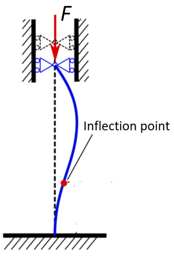
Beam and boundary conditions for Example 1
Figure 2. Geometry, boundary conditions and reference compressive load for Example 1.

The Euler critical load is:

Fcr=20.19EIL2=53840 NF_{\rm cr}=20.19\frac{EI}{L^2}=53840\ \mathrm{N}

The following table compares the first buckling load obtained with the three beam elements.

ElementsEuler–Bernoulli (N)Timoshenko isoparametric (N)Timoshenko cubic (N)
1053846.556151.253729.5
2053842.254251.553723.5
3053842.053948.653722.9
4053842.053847.453722.8
5053841.953801.753722.8
10053841.953742.053722.7
20053841.953727.553722.6

Timoshenko-based finite elements lead to a slightly smaller critical load because they also account for shear deformation. For slender beams, this effect becomes negligible and the Timoshenko solution approaches the Euler–Bernoulli result. The convergence of the two-node isoparametric element is slower than that of the third-degree element.

Figure 3. First buckling eigenvector for Example 1.

08

Example 2

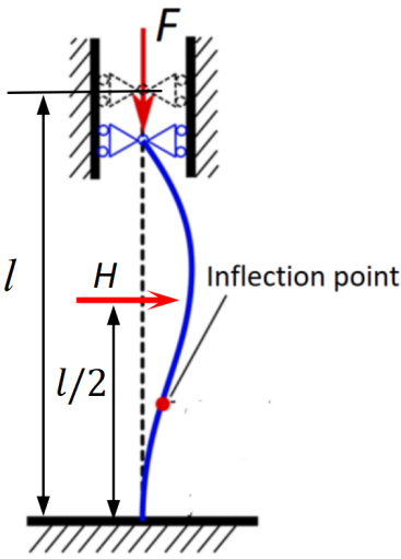
The same beam is subjected to an axial compressive force and a small transverse force HH.

Beam loading for Example 2
Figure 4. Loading and boundary conditions for the geometrically nonlinear verification.

This is not a buckling eigenvalue problem. It is a large-displacement analysis solved using the Updated Lagrangian formulation.

The purpose of this example is to verify the linear buckling prediction through a geometrically nonlinear equilibrium path. As the lateral load HH tends to zero, the equilibrium curves approach the critical load obtained from the eigenvalue buckling analysis.

Figure 5. Nonlinear equilibrium curves for decreasing values of the transverse load HH.

09

Example 3

The structure consists of two beams with square 20×20 mm20\times20\ \mathrm{mm} cross-sections. Young's modulus is E=200000 MPaE=200000\ \mathrm{MPa}, and Poisson's ratio is ν=0.25\nu=0.25. The geometry, supports and loading are shown below.
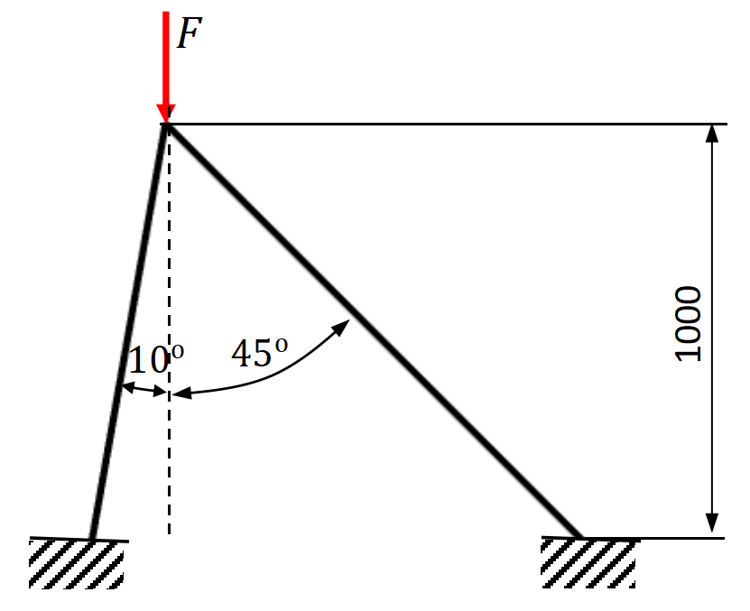
Two-member frame for Example 3
Figure 6. Geometry, boundary conditions and loading for Example 3.
Figure 7. First buckling mode. MATLAB: 75547.3 N; ANSYS: 75657.8 N.
Figure 8. Second buckling mode. MATLAB: 172986.9 N; ANSYS: 173530.1 N.

10

Reference

[1] Timoshenko, S.P., Gere, J.M., Theory of Elastic Stability, McGraw-Hill, 1985.