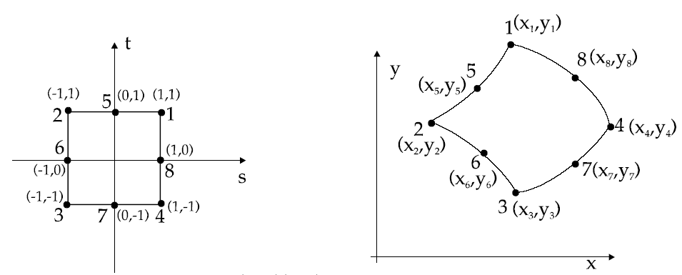
9.6. Isoparametric 8-node quadrilateral finite element

Element and hypotheses

Small strains

Small displacements

Linear elastic material

The theory is well known, see for instance [1]. This finite element has eight nodes and two degrees of freedom per node, giving 16 element displacement degrees of freedom. The theory is presented briefly, following the same development as for the Q4 element in Section 9.4.

\boldsymbol f_{el}=\boldsymbol k_{el}\boldsymbol u_{el},\qquad\boldsymbol f_{el}=\begin{Bmatrix}X_1\\Y_1\\X_2\\Y_2\\X_3\\Y_3\\\vdots\\X_8\\Y_8\end{Bmatrix},\qquad\boldsymbol u_{el}=\begin{Bmatrix}u_1\\v_1\\u_2\\v_2\\u_3\\v_3\\\vdots\\u_8\\v_8\end{Bmatrix}

Here $\boldsymbol f_{el}$ is the nodal-force vector, $\boldsymbol u_{el}$ is the nodal-displacement vector, and $\boldsymbol k_{el}$ is the element stiffness matrix:

\boldsymbol u_{el}\in\mathbb R^{16\times1},\qquad\boldsymbol k_{el}\in\mathbb R^{16\times16}.

Natural coordinates and interpolation

Q8 natural and Cartesian coordinates with corner nodes 1 to 4 and midside nodes 5 to 8 — The Q8 element in natural coordinates (left) and Cartesian coordinates (right), with the nodal numbering used below.

Interpolation functions:

\begin{aligned}N_1&=\frac{(1+s)(1+t)}4-\frac12N_5-\frac12N_8,\\N_2&=\frac{(1-s)(1+t)}4-\frac12N_5-\frac12N_6,\\N_3&=\frac{(1-s)(1-t)}4-\frac12N_6-\frac12N_7,\\N_4&=\frac{(1+s)(1-t)}4-\frac12N_7-\frac12N_8.\end{aligned}

\begin{aligned}N_5&=\frac{(1-s^2)(1+t)}2,&N_6&=\frac{(1-t^2)(1-s)}2,\\N_7&=\frac{(1-s^2)(1-t)}2,&N_8&=\frac{(1-t^2)(1+s)}2.\end{aligned}

The same interpolation functions are used for coordinates as for displacements:

\begin{Bmatrix}x(s,t)\\y(s,t)\end{Bmatrix}=\sum_{i=1}^8N_i(s,t)\begin{Bmatrix}x_i\\y_i\end{Bmatrix},\qquad\begin{Bmatrix}u(s,t)\\v(s,t)\end{Bmatrix}=\sum_{i=1}^8N_i(s,t)\begin{Bmatrix}u_i\\v_i\end{Bmatrix}.

Strains and Jacobian

Strains:

\boldsymbol\varepsilon=\begin{Bmatrix}\varepsilon_x\\\varepsilon_y\\\gamma_{xy}\end{Bmatrix}=\begin{Bmatrix}\dfrac{\partial u}{\partial x}\\\dfrac{\partial v}{\partial y}\\\dfrac{\partial u}{\partial y}+\dfrac{\partial v}{\partial x}\end{Bmatrix}=\begin{Bmatrix}\dfrac{\partial u}{\partial x}\\0\\\dfrac{\partial u}{\partial y}\end{Bmatrix}+\begin{Bmatrix}0\\\dfrac{\partial v}{\partial y}\\\dfrac{\partial v}{\partial x}\end{Bmatrix}.

\boldsymbol\varepsilon=\begin{bmatrix}1&0\\0&0\\0&1\end{bmatrix}\begin{Bmatrix}\dfrac{\partial u}{\partial x}\\\dfrac{\partial u}{\partial y}\end{Bmatrix}+\begin{bmatrix}0&0\\0&1\\1&0\end{bmatrix}\begin{Bmatrix}\dfrac{\partial v}{\partial x}\\\dfrac{\partial v}{\partial y}\end{Bmatrix}.

With:

\begin{Bmatrix}\dfrac{\partial u}{\partial x}\\\dfrac{\partial u}{\partial y}\end{Bmatrix}=\boldsymbol J^{-1}\begin{Bmatrix}\dfrac{\partial u}{\partial s}\\\dfrac{\partial u}{\partial t}\end{Bmatrix},\qquad\begin{Bmatrix}\dfrac{\partial v}{\partial x}\\\dfrac{\partial v}{\partial y}\end{Bmatrix}=\boldsymbol J^{-1}\begin{Bmatrix}\dfrac{\partial v}{\partial s}\\\dfrac{\partial v}{\partial t}\end{Bmatrix}.

$\boldsymbol J$ is the Jacobian:

\boldsymbol J(s,t)=\begin{bmatrix}\dfrac{\partial x}{\partial s}&\dfrac{\partial y}{\partial s}\\\dfrac{\partial x}{\partial t}&\dfrac{\partial y}{\partial t}\end{bmatrix}.

Using interpolation functions:

\boldsymbol J(s,t)=\boldsymbol H(s,t)\begin{bmatrix}x_1&y_1\\x_2&y_2\\\vdots&\vdots\\x_8&y_8\end{bmatrix},

\boldsymbol H(s,t)=\begin{bmatrix}\dfrac{\partial N_1}{\partial s}&\dfrac{\partial N_2}{\partial s}&\cdots&\dfrac{\partial N_8}{\partial s}\\\dfrac{\partial N_1}{\partial t}&\dfrac{\partial N_2}{\partial t}&\cdots&\dfrac{\partial N_8}{\partial t}\end{bmatrix}.

Therefore:

\boldsymbol\varepsilon=\begin{bmatrix}1&0\\0&0\\0&1\end{bmatrix}\boldsymbol J^{-1}\begin{Bmatrix}\dfrac{\partial u}{\partial s}\\\dfrac{\partial u}{\partial t}\end{Bmatrix}+\begin{bmatrix}0&0\\0&1\\1&0\end{bmatrix}\boldsymbol J^{-1}\begin{Bmatrix}\dfrac{\partial v}{\partial s}\\\dfrac{\partial v}{\partial t}\end{Bmatrix}.

Strain-displacement matrix

Using the interpolation functions again:

\begin{Bmatrix}\dfrac{\partial u}{\partial s}\\\dfrac{\partial u}{\partial t}\end{Bmatrix}=\boldsymbol H(s,t)\begin{Bmatrix}u_1\\u_2\\\vdots\\u_8\end{Bmatrix},\qquad\begin{Bmatrix}\dfrac{\partial v}{\partial s}\\\dfrac{\partial v}{\partial t}\end{Bmatrix}=\boldsymbol H(s,t)\begin{Bmatrix}v_1\\v_2\\\vdots\\v_8\end{Bmatrix}.

Thus:

\boldsymbol\varepsilon=\begin{bmatrix}1&0\\0&0\\0&1\end{bmatrix}\boldsymbol b\begin{Bmatrix}u_1\\u_2\\\vdots\\u_8\end{Bmatrix}+\begin{bmatrix}0&0\\0&1\\1&0\end{bmatrix}\boldsymbol b\begin{Bmatrix}v_1\\v_2\\\vdots\\v_8\end{Bmatrix},

where:

\boldsymbol b=\boldsymbol J^{-1}\boldsymbol H=\begin{bmatrix}b_{11}&b_{12}&\cdots&b_{18}\\b_{21}&b_{22}&\cdots&b_{28}\end{bmatrix}.

Collecting the nodal displacement components gives:

\boldsymbol\varepsilon=\begin{Bmatrix}\varepsilon_x\\\varepsilon_y\\\gamma_{xy}\end{Bmatrix}=\boldsymbol B\boldsymbol u_{el}.

\boldsymbol B(s,t)=\begin{bmatrix}b_{11}&0&b_{12}&0&b_{13}&0&b_{14}&0&b_{15}&0&b_{16}&0&b_{17}&0&b_{18}&0\\0&b_{21}&0&b_{22}&0&b_{23}&0&b_{24}&0&b_{25}&0&b_{26}&0&b_{27}&0&b_{28}\\b_{21}&b_{11}&b_{22}&b_{12}&b_{23}&b_{13}&b_{24}&b_{14}&b_{25}&b_{15}&b_{26}&b_{16}&b_{27}&b_{17}&b_{28}&b_{18}\end{bmatrix}.

\boldsymbol B\in\mathbb R^{3\times16}.

Constitutive law and stiffness matrix

The stiffness matrix for the finite element is:

\boxed{\boldsymbol k_{el}=h\int_A\boldsymbol B^T\boldsymbol D\boldsymbol B\,dA}

$E$ is Young’s modulus, $\nu$ is Poisson’s ratio, and $h$ is the thickness of the finite element. For the plane stress state:

\boldsymbol D=\frac{E}{1-\nu^2}\begin{bmatrix}1&\nu&0\\\nu&1&0\\0&0&\dfrac{1-\nu}{2}\end{bmatrix}.

Since $\boldsymbol B$ is a function of $s$ and $t$ , it is more convenient to work in natural coordinates. Consequently, for a positively oriented mapping:

\boxed{\boldsymbol k_{el}=h\int_{-1}^{1}\int_{-1}^{1}\boldsymbol B(s,t)^T\boldsymbol D\boldsymbol B(s,t)\det\boldsymbol J(s,t)\,ds\,dt}

$\det\boldsymbol J(s,t)$ is the determinant of the Jacobian.

Gauss quadrature

The third-order one-dimensional Gauss rule used in the program is:

$i$	Gauss coordinate	Weight
1	$-\sqrt{0.6}$	$5/9$
2	$0$	$8/9$
3	$+\sqrt{0.6}$	$5/9$

The two-dimensional rule is the tensor product of this one-dimensional rule. Each coordinate is paired with all three coordinates in the other direction, giving $3\times3=9$ Gauss points per element. The weight of a pair is $w_iw_j$ :

\boldsymbol k_{el}\approx h\sum_{j=1}^3\sum_{i=1}^3 w_iw_j\boldsymbol B(s_i,t_j)^T\boldsymbol D\boldsymbol B(s_i,t_j)\left|\det\boldsymbol J(s_i,t_j)\right|.

MATLAB example

A simple MATLAB program can be downloaded below. Run main.m; it calls the following subprograms:

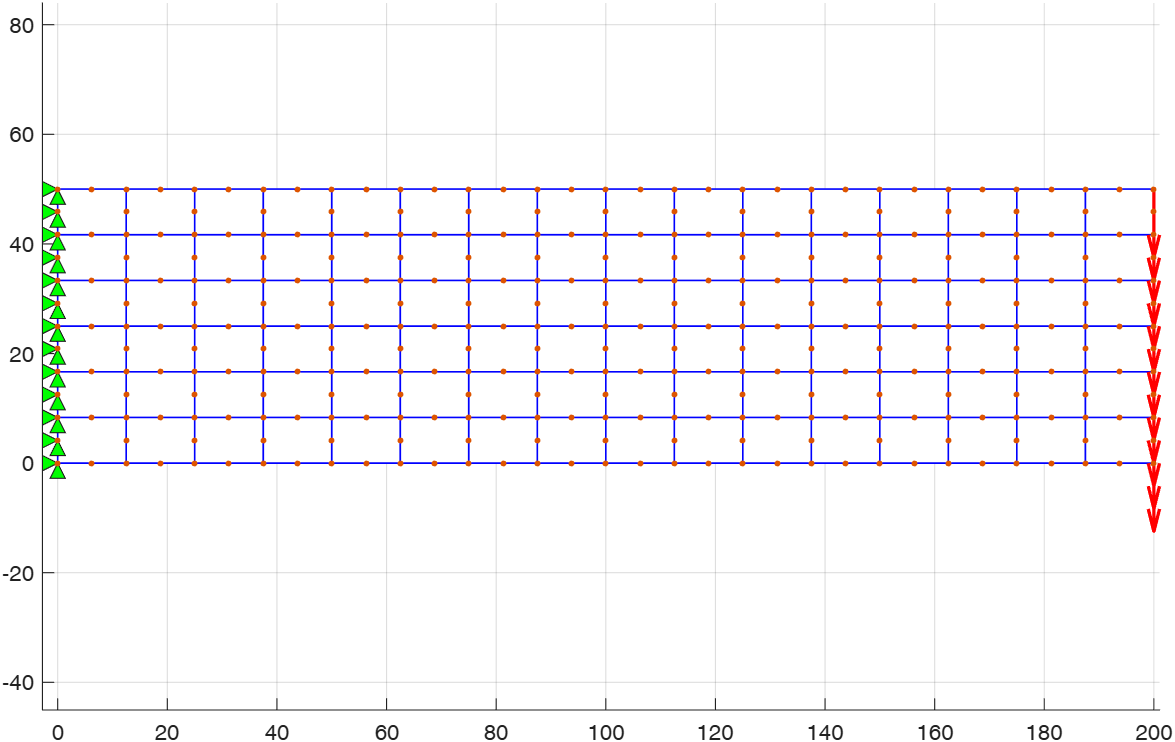
gen generates the mesh for a cantilever clamped at $x=0$ ( $u=0, v=0$ ) and loaded with a force uniformly distributed on the other end ( $x=L$ ). See the program for all input data and further explanations.
plane2d8 generates the stiffness matrices of all finite elements, performs the assembling process, imposes boundary conditions, and solves the linear system for nodal displacements.
plot_disp plots the displacement colour map.
plot_stress plots the stress colour map.

L=200\ \mathrm{mm},\quad H=50\ \mathrm{mm},\quad h=5\ \mathrm{mm},

E=2.1\times10^5\ \mathrm{MPa},\quad\nu=0.3,\quad F=1000\ \mathrm N,\quad n_L=16,\quad n_H=6.

The results are calculated for a mesh of 16 Q8 elements along the beam and 6 elements through its height: 96 finite elements, 333 nodes, and 666 equations. The total applied vertical force is $-1000\ \mathrm N$ .

Q8 mesh, constraints and distributed load — **Figure 1.** Q8 cantilever mesh, boundary conditions, and distributed free-end load, generated by `gen.m`.

Displacement results

The following maps are generated by the Q8 program. Displacements are in millimetres; the displacement plotting scale is 1.

Q8 MATLAB result map, Figure 2 — **Figure 2.** Horizontal displacement $u$ . $u_{\min}=-0.04595\ \mathrm{mm},\quad u_{\max}=0.04595\ \mathrm{mm}$ .

Q8 MATLAB result map, Figure 3 — **Figure 3.** Vertical displacement $v$ . $v_{\min}=-0.2545\ \mathrm{mm},\quad v_{\max}=0$ .

For comparison, the magnitude of the free-end displacement predicted by the Timoshenko beam model is:

|v|_{\max}=\frac{FL^3}{3EI}+1.2\frac{FL}{GA}=0.2557\ \mathrm{mm},\qquad I=\frac{hH^3}{12},\quad A=hH,\quad G=\frac{E}{2(1+\nu)}.

The Q8 result is very close to the beam solution: the difference in the maximum displacement magnitude is about 0.46%. The finite element displacement is negative because the applied force acts in the negative vertical direction.

Stress results

For plotting, stresses are evaluated at the eight element nodes and averaged at nodes shared by adjacent elements. The stress maps use the default displacement scale 0 and are therefore shown on the undeformed configuration. Stresses are in MPa.

Q8 MATLAB result map, Figure 4 — **Figure 4.** Normal stress $\sigma_x$ . $\sigma_{x,\min}=-113.409\ \mathrm{MPa},\quad\sigma_{x,\max}=113.409\ \mathrm{MPa}$ .

Von Mises stress: $\sigma_{\mathrm{VM},\min}=2.295\ \mathrm{MPa},\quad\sigma_{\mathrm{VM},\max}=106.477\ \mathrm{MPa}$ .

Comparison with Q4

The same cantilever geometry, material, thickness, and resultant loading are used in Section 9.4. Both programs were run in MATLAB R2026a Update 4. The comparison uses the actual results of the Q4 mesh with 40 elements along the length and 16 through the height:

Quantity	Q4 — Section 9.4	Q8 — Section 9.6
Elements	640	96
Nodes	697	333
Equations	1394	666
$u_{\min}\ (\mathrm{mm})$	-0.04574	-0.04595
$u_{\max}\ (\mathrm{mm})$	0.04574	0.04595
$v_{\min}\ (\mathrm{mm})$	-0.2535	-0.2545
$\sigma_{x,\min}\ (\mathrm{MPa})$	-115.217	-113.409
$\sigma_{x,\max}\ (\mathrm{MPa})$	115.217	113.409
$\sigma_{\mathrm{VM},\min}\ (\mathrm{MPa})$	4.442	2.295
$\sigma_{\mathrm{VM},\max}\ (\mathrm{MPa})$	109.174	106.477

Q8 obtains essentially the same displacement solution and comparable stress levels with a substantially smaller discretization than Q4, because its higher-order interpolation represents bending more efficiently.

Q8 has midside nodes and quadratic interpolation along its edges. It can represent curved displacement fields and stress gradients more accurately than a bilinear Q4 element, which is particularly useful in bending-dominated problems. Curved boundaries can also be represented more accurately. The cost per element is higher, but fewer elements are often required for a comparable solution.

Programs and download

main.m

clear
gen
plane2d8
plot_disp
plot_stress

MQ8 MATLAB programFive MATLAB files and README · tested in MATLAB R2026a Update 4Download ZIP

Reference

[1] Carlos A. Felippa, Introduction to Finite Element Methods, University of Colorado, Boulder, Colorado.