8.2 2D Isoparametric Beam Element

Updated Lagrangian formulation

For completeness, the Updated Lagrangian formulation used in this section is summarized below. Configuration $i$ is known and becomes the reference configuration for the next load step. Configuration $i+1$ is the unknown target configuration. Stresses, strains, and displacement increments in the target configuration are evaluated with respect to configuration $i$ ; derivatives and integrals are likewise evaluated with respect to the previous configuration.

StrainSmall

MaterialLinear elastic

DisplacementLarge

ElementStraight, prismatic, two-node

Beam modelTimoshenko

FormulationUpdated Lagrangian

Reference configuration

The current configuration at load step $i$ is known.
It serves as the reference configuration while solving load step $i+1$ .
After convergence, the newly obtained geometry becomes the reference for the following load step.

Total and Updated Lagrangian descriptions

The distinction between the two descriptions is summarized below [1].

Total Lagrangian (TL)	Updated Lagrangian (UL)
The initial configuration is the reference configuration. Quantities in the target configuration are referred to the initial configuration. Derivatives and integrals are evaluated with respect to the initial configuration.	The previous/current configuration is the reference configuration. Quantities in the target configuration are referred to the previous configuration. Derivatives and integrals are evaluated with respect to the previous configuration.

Configurations and coordinate frames

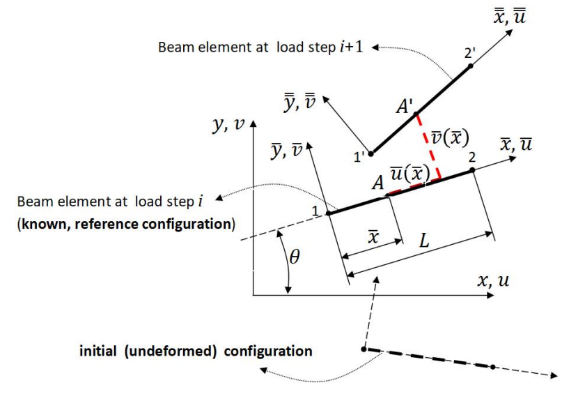
The global frame $(x,y)$ is common to all load steps. The known beam configuration at load step $i$ is described by the local frame $(\bar{x},\bar{y})$ , which becomes the reference frame for the unknown configuration at $i+1$ .

The local displacements $\bar u(\bar x)$ and $\bar v(\bar x)$ shown between configurations $i$ and $i+1$ are displacement increments for the current load step, not total displacements measured from the initial undeformed configuration. Generalized strains are evaluated in the local frame, while nodal displacement increments are assembled in the fixed global frame.

Updated Lagrangian beam element in the known reference configuration and the next target configuration — Figure 1. Initial configuration, known current configuration at load step $i$ , and target configuration at load step $i+1$ . The barred local displacements are increments for the current load step.

Deformation energy and generalized strains

Using one Gauss point for each two-node isoparametric beam element, the deformation energy of the complete structure at load step $i+1$ is:

U_{i+1}=\frac{1}{2}\sum L\left(EA\,\varepsilon_{0,i+1}^{2}+EI\,\kappa_{i+1}^{2}+GA_0\,\beta_{i+1}^{2}\right)

Equivalently, in terms of the known generalized strains at configuration $i$ and the unknown increments for the current load step,

U_{i+1}=\frac{1}{2}\sum L\left[EA\left(\varepsilon_{0,i}+\Delta\varepsilon_0\right)^2+EI\left(\kappa_i+\Delta\kappa\right)^2+GA_0\left(\beta_i+\Delta\beta\right)^2\right]

The summation sign denotes assembly over all beam elements. The three generalized strain measures satisfy

\left\{\begin{aligned}\varepsilon_{0,i+1}&=\varepsilon_{0,i}+\Delta\varepsilon_0\\[6pt]\kappa_{i+1}&=\kappa_i+\Delta\kappa\\[6pt]\beta_{i+1}&=\beta_i+\Delta\beta\end{aligned}\right.

Here $\varepsilon_0$ is the axial strain, $\kappa$ is the curvature, and $\beta$ is the Timoshenko shear angle. The associated generalized stress resultants are the axial force, bending moment, and shear force: $N$ , $M$ , and $T$ .

Derivatives during a load step

During the solution of load step $i+1$ , the quantities $\varepsilon_{0,i}$ , $\kappa_i$ , and $\beta_i$ are known and remain constant. Their derivatives with respect to the unknown element displacement-increment vector therefore involve only the corresponding increments:

\begin{aligned}\frac{\partial\varepsilon_{0,i+1}}{\partial\Delta\boldsymbol u_{el}}&=\frac{\partial\Delta\varepsilon_0}{\partial\Delta\boldsymbol u_{el}},&\qquad \frac{\partial^2\varepsilon_{0,i+1}}{\partial\Delta\boldsymbol u_{el}^{2}}&=\frac{\partial^2\Delta\varepsilon_0}{\partial\Delta\boldsymbol u_{el}^{2}}\\[8pt]\frac{\partial\kappa_{i+1}}{\partial\Delta\boldsymbol u_{el}}&=\frac{\partial\Delta\kappa}{\partial\Delta\boldsymbol u_{el}},&\qquad \frac{\partial^2\kappa_{i+1}}{\partial\Delta\boldsymbol u_{el}^{2}}&=\frac{\partial^2\Delta\kappa}{\partial\Delta\boldsymbol u_{el}^{2}}\\[8pt]\frac{\partial\beta_{i+1}}{\partial\Delta\boldsymbol u_{el}}&=\frac{\partial\Delta\beta}{\partial\Delta\boldsymbol u_{el}},&\qquad \frac{\partial^2\beta_{i+1}}{\partial\Delta\boldsymbol u_{el}^{2}}&=\frac{\partial^2\Delta\beta}{\partial\Delta\boldsymbol u_{el}^{2}}\end{aligned}

From the TL program to the UL program

Only a few modifications are required to extend the Total Lagrangian beam formulations and programs presented in Sections 7.1 and 7.2 to the present Updated Lagrangian formulation. The arrays store the three generalized quantities $\varepsilon_0,\kappa,\beta$ and their associated resultants:

main.mGeneralized-strain and stress history

strn=zeros(nel,3,nstep+1);
stress=zeros(nel,3,nstep+1);

The current increment is reset immediately after the load-step loop begins, and the geometry update is called after the Newton–Raphson loop:

main.mIncremental solution and total displacement

for istep=1:nstep
    S=zeros(neq,1);
    ...
    updt
    St(:,istep+1)=St(:,istep)+S;
end

The generalized stress resultants are evaluated after the load-step solution:

main.mAxial force, bending moment, and shear force

stress(:,1,:)=EA*strn(:,1,:);
stress(:,2,:)=EI*strn(:,2,:);
stress(:,3,:)=GA*strn(:,3,:);

Element assembly and configuration update

After the incremental kinematics are evaluated in deriv.m, the generalized strains accumulated in the preceding configuration are added:

stiff.mGeneralized-strain accumulation

ep=ep+strn(ie,1,istep);
ca=ca+strn(ie,2,istep);
be=be+strn(ie,3,istep);

The following line is added immediately before the two assembly statements:

stiff.mStorage and global assembly

strn(ie,1:3,istep+1)=[ep ca be];
F(ip)=F(ip)+R'*fel;
K(ip,ip)=K(ip,ip)+R'*kel*R;

The essential updt.m subprogram updates the nodal coordinates

updt.mGeometry update

x=x+S(1:3:neq);
y=y+S(2:3:neq);

It then recomputes every element length and rotation matrix Rt. Thus, after each converged load step, the newly obtained configuration becomes the reference configuration for the following load step.

Accuracy and load-step independence

Important remark

Unlike the Euler–Bernoulli incremental approximation used in Section 8.1, the present isoparametric Timoshenko formulation does not rely on the same small-displacement-increment approximation. Within the adopted beam model, finite element discretization, and numerical tolerances, the converged solution should therefore be essentially independent of the chosen number of load steps. Several steps may nevertheless help trace the equilibrium path and improve convergence.

For a single load step, the reference configuration is still the initial configuration; therefore, the present UL formulation reduces to the corresponding TL formulation.

Example 1 — moment-loaded cantilever

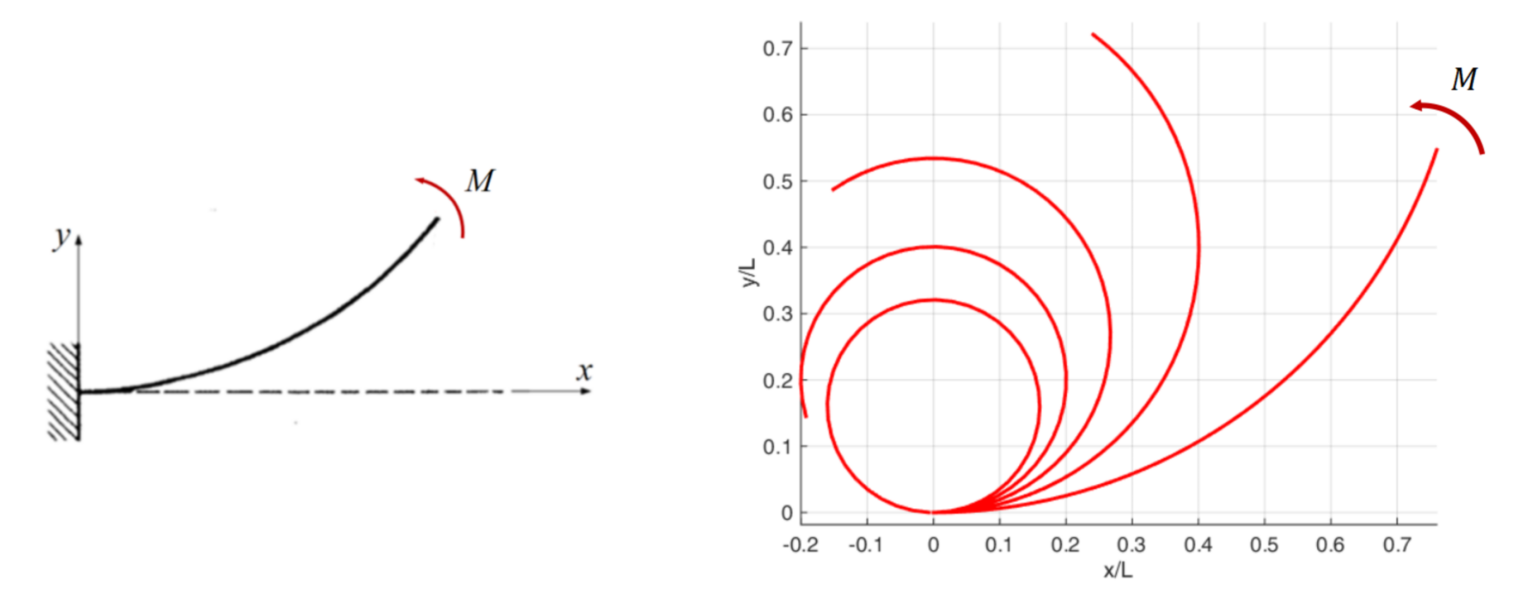
A cantilever beam of length $L_b=100\ \mathrm{mm}$ has a rectangular cross-section $5\ \mathrm{mm}\times1\ \mathrm{mm}$ (width × thickness), Young's modulus $E=2\times10^5\ \mathrm{MPa}$ , and an applied free-end moment $M=5236\ \mathrm{Nmm}$ .

The analytical maximum rotation is:

\varphi_{\max}=\frac{ML_b}{EI}=\frac{5236\cdot100}{2\times10^5\cdot5\cdot1^3/12}=2\pi\ \mathrm{rad}

The figure shows five equidistant load steps. The same example appears in Section 8.1 and illustrates how the Euler–Bernoulli incremental formulation approaches this solution when sufficiently small displacement increments are used.

Moment-loaded cantilever and five equidistant deformed configurations — Figure 2. Moment-loaded cantilever and five equidistant load steps. Coordinates are normalized by the beam length as $x/L_b$ and $y/L_b$ .

Example 2 — Mattiasson benchmark

This large-deflection beam-frame benchmark is taken from Mattiasson [2], where reference solutions are obtained using elliptic integrals. The downloadable MATLAB package is intentionally configured for this example.

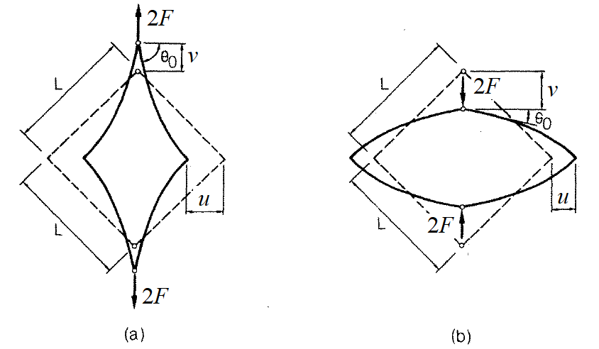
Two symmetric Mattiasson large-deflection beam-frame benchmark configurations — Figure 3. Geometry, loading, and displacement measures for the two Mattiasson benchmark cases [2].

To reconstruct the complete symmetric structure, activate the two cl=...; plt commands in main.m and comment the neighboring direct plotting commands, as explained in the README. The resulting deformed configurations and normalized response curves show very good agreement with the elliptic-integral reference values.

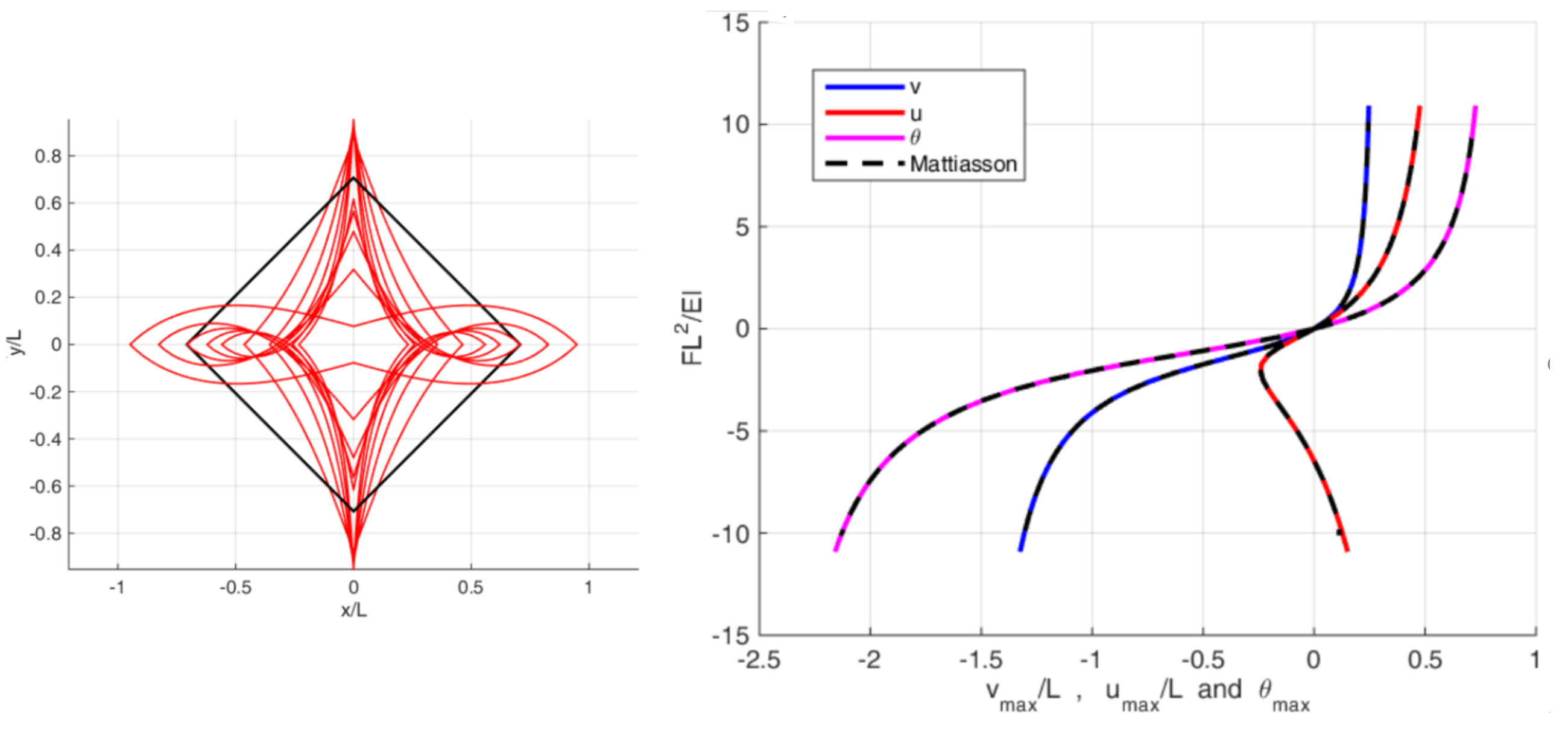
Symmetric deformed configurations and normalized response curves compared with Mattiasson — Figure 4. Symmetric deformed configurations and normalized load–displacement curves. Solid curves are obtained with the isoparametric Timoshenko beam element; dashed curves are the elliptic-integral reference values from [2].

Remark 1

Mattiasson's benchmark uses an Euler–Bernoulli bending model, whereas the present finite element formulation uses the Timoshenko beam model and therefore also allows axial and shear deformation. The results are practically identical here because axial and shear deformations are negligible for this very slender leaf spring.

Remark 2

The Updated Lagrangian description naturally leads to an incremental procedure, which is especially convenient for problems such as elastoplastic analysis. For a single load step, the initial configuration remains the reference and the present UL formulation reduces to its TL counterpart.

MATLAB package

The package contains seven MATLAB files and a README. Its input data are configured for Example 2; no separate Example 1 input file is distributed.

MATLAB verification

Tested in MATLAB 26.1 (R2026a). All 10 load steps converged. The final load step required 5 Newton–Raphson iterations and reached a convergence measure of $1.03\times10^{-7}$ . No additional toolbox is required.

MUpdated Lagrangian isoparametric beam package7 MATLAB files and README · configured for Example 2 · tested in R2026aDownload ZIP

References

E. Chatzi and K. Agathos, Linearized weak form and total Lagrangian formulation of a bar element, Institute of Structural Engineering, ETH Zurich, Lecture 3, 3 October 2019.
K. Mattiasson, Numerical results from large deflection beam and frame problems analysed by means of elliptic integrals, International Journal for Numerical Methods in Engineering, 16, 145–153, 1981.