26.2. Isoparametric 20-node hexahedral finite element

StrainSmall

DisplacementLarge

MaterialLinear elastic

Introduction

The Total Lagrangian formulation developed in Section 26.1 can be applied directly to the 20-node isoparametric hexahedral finite element. Therefore, only the modifications resulting from the higher-order interpolation are presented here. The geometry, node numbering, natural coordinates and interpolation functions of the HEX20 element were presented in Section 25.3.

The HEX20 element has 20 nodes and three displacement DOFs per node, therefore 60 element DOFs:

\htmlClass{fea-math-bold-italic}{\boldsymbol{u}}_{el}=\begin{Bmatrix}u_1&v_1&w_1&\cdots&u_{20}&v_{20}&w_{20}\end{Bmatrix}^{T}.

Element matrices

The nodal coordinates, measured in the initial undeformed configuration, are collected in the following matrix:

\htmlClass{fea-math-bold-italic}{\boldsymbol{x}}_{el}=\begin{bmatrix}x_1&y_1&z_1\\x_2&y_2&z_2\\\vdots&\vdots&\vdots\\x_{20}&y_{20}&z_{20}\end{bmatrix}\in\mathbb R^{20\times3}.

The natural-coordinate derivatives of the interpolation functions define:

\htmlClass{fea-math-bold-italic}{\boldsymbol{H}}(s,t,r)=\begin{bmatrix}N_{1,s}&N_{2,s}&\cdots&N_{20,s}\\N_{1,t}&N_{2,t}&\cdots&N_{20,t}\\N_{1,r}&N_{2,r}&\cdots&N_{20,r}\end{bmatrix},

\htmlClass{fea-math-bold-italic}{\boldsymbol{J}}_0=\htmlClass{fea-math-bold-italic}{\boldsymbol{H}}\htmlClass{fea-math-bold-italic}{\boldsymbol{x}}_{el},\qquad\htmlClass{fea-math-bold-italic}{\boldsymbol{b}}=\htmlClass{fea-math-bold-italic}{\boldsymbol{J}}_0^{-1}\htmlClass{fea-math-bold-italic}{\boldsymbol{H}}.

The interpolation functions are given in Section 25.3. The subprogram shape20.m supplies these functions and their natural-coordinate derivatives; $\htmlClass{fea-math-bold-italic}{\boldsymbol b}$ contains their Cartesian derivatives with respect to the initial configuration.

The dimensions of the strain–displacement and geometric matrices become:

\htmlClass{fea-math-bold-italic}{\boldsymbol B}_0,\;\htmlClass{fea-math-bold-italic}{\boldsymbol B}_L,\;\htmlClass{fea-math-bold-italic}{\boldsymbol B}\in\mathbb R^{6\times60},

\htmlClass{fea-math-bold-italic}{\boldsymbol G}_x,\htmlClass{fea-math-bold-italic}{\boldsymbol G}_y,\htmlClass{fea-math-bold-italic}{\boldsymbol G}_z,\htmlClass{fea-math-bold-italic}{\boldsymbol G}_{xy},\htmlClass{fea-math-bold-italic}{\boldsymbol G}_{yz},\htmlClass{fea-math-bold-italic}{\boldsymbol G}_{zx}\in\mathbb R^{60\times60}.

As in Section 26.1:

\htmlClass{fea-math-bold-italic}{\boldsymbol B}=\htmlClass{fea-math-bold-italic}{\boldsymbol B}_0+\htmlClass{fea-math-bold-italic}{\boldsymbol B}_L.

The finite-element tangent stiffness matrix remains:

\boxed{\htmlClass{fea-math-bold-italic}{\boldsymbol k}_{el}=\htmlClass{fea-math-bold-italic}{\boldsymbol k}_{M_{el}}+\htmlClass{fea-math-bold-italic}{\boldsymbol k}_{G_{el}}},

where $M$ means material and $G$ means geometric. The Green–Lagrange strain development, the definition of the geometric matrices, virtual work and the Newton–Raphson method are unchanged; their complete derivation is given in Section 26.1.

Numerical integration

An important difference from HEX8 is the integration rule. HEX20 uses:

3\times3\times3=27\quad\mathit{Gauss points}.

In each natural-coordinate direction, the Gauss coordinates and weights are:

Coordinate	Weight
$-\sqrt{3/5}$	$5/9$
$0$	$8/9$
$+\sqrt{3/5}$	$5/9$

The three-dimensional Gauss weight is the product of the three one-dimensional weights:

w_g=w_s w_t w_r,

where $w_s,w_t,w_r$ are the weights $5/9,8/9,5/9$ associated, respectively, with the coordinates $-\sqrt{3/5},0,+\sqrt{3/5}$ in each natural-coordinate direction. The four possible products are:

\begin{aligned}(5/9)^3&=125/729,\\(5/9)^2(8/9)&=200/729,\\(5/9)(8/9)^2&=320/729,\\(8/9)^3&=512/729.\end{aligned}

Thus:

\htmlClass{fea-math-bold-italic}{\boldsymbol f}_{el}=\sum_{g=1}^{27}w_g\,\htmlClass{fea-math-bold-italic}{\boldsymbol B}^T\htmlClass{fea-math-bold-italic}{\boldsymbol{\sigma}}\,\mathop{\mathit{det}}(\htmlClass{fea-math-bold-italic}{\boldsymbol J}_0),

\htmlClass{fea-math-bold-italic}{\boldsymbol k}_{el}=\sum_{g=1}^{27}w_g\left[\htmlClass{fea-math-bold-italic}{\boldsymbol B}^T\htmlClass{fea-math-bold-italic}{\boldsymbol D}\htmlClass{fea-math-bold-italic}{\boldsymbol B}+\sigma_x\htmlClass{fea-math-bold-italic}{\boldsymbol G}_x+\sigma_y\htmlClass{fea-math-bold-italic}{\boldsymbol G}_y+\sigma_z\htmlClass{fea-math-bold-italic}{\boldsymbol G}_z+\tau_{xy}\htmlClass{fea-math-bold-italic}{\boldsymbol G}_{xy}+\tau_{yz}\htmlClass{fea-math-bold-italic}{\boldsymbol G}_{yz}+\tau_{zx}\htmlClass{fea-math-bold-italic}{\boldsymbol G}_{zx}\right]\mathop{\mathit{det}}(\htmlClass{fea-math-bold-italic}{\boldsymbol J}_0).

Example

The same cantilever as in Section 26.1 is analysed, with the same dimensions, material properties and loads:

L=200\,\mathit{mm},\qquad t=20\,\mathit{mm},\qquad h=5\,\mathit{mm},

E=2\times10^5\,\mathit{MPa},\qquad\nu=0.3,\qquad F_1=4000\,\mathit N,\qquad F_2=4F_1.

The HEX20 mesh used in the program contains:

30\times4\times2=240\quad\mathit{HEX20 elements},

1597\quad\mathit{nodes},\qquad4791\quad\mathit{equations}.

Figure 1. Deformed HEX20 cantilever. Coordinates are in millimetres. Drag to rotate; Zoom is initially OFF. Reset view restores the initial camera.

The MATLAB program implementing the Total Lagrangian formulation with HEX20 can be downloaded below. Run main.m. The subprogram shape20.m, already used in Section 25.3, supplies the interpolation functions and their natural-coordinate derivatives.

MMATLAB — Hex20_TL.zipEight MATLAB files and README.md.Download ZIP

The ANSYS macro used for comparison can be downloaded here:

AANSYS — Hex20.macCantilever comparison macro; millimetres, newtons and MPa.Download MAC

Results and comparison with ANSYS

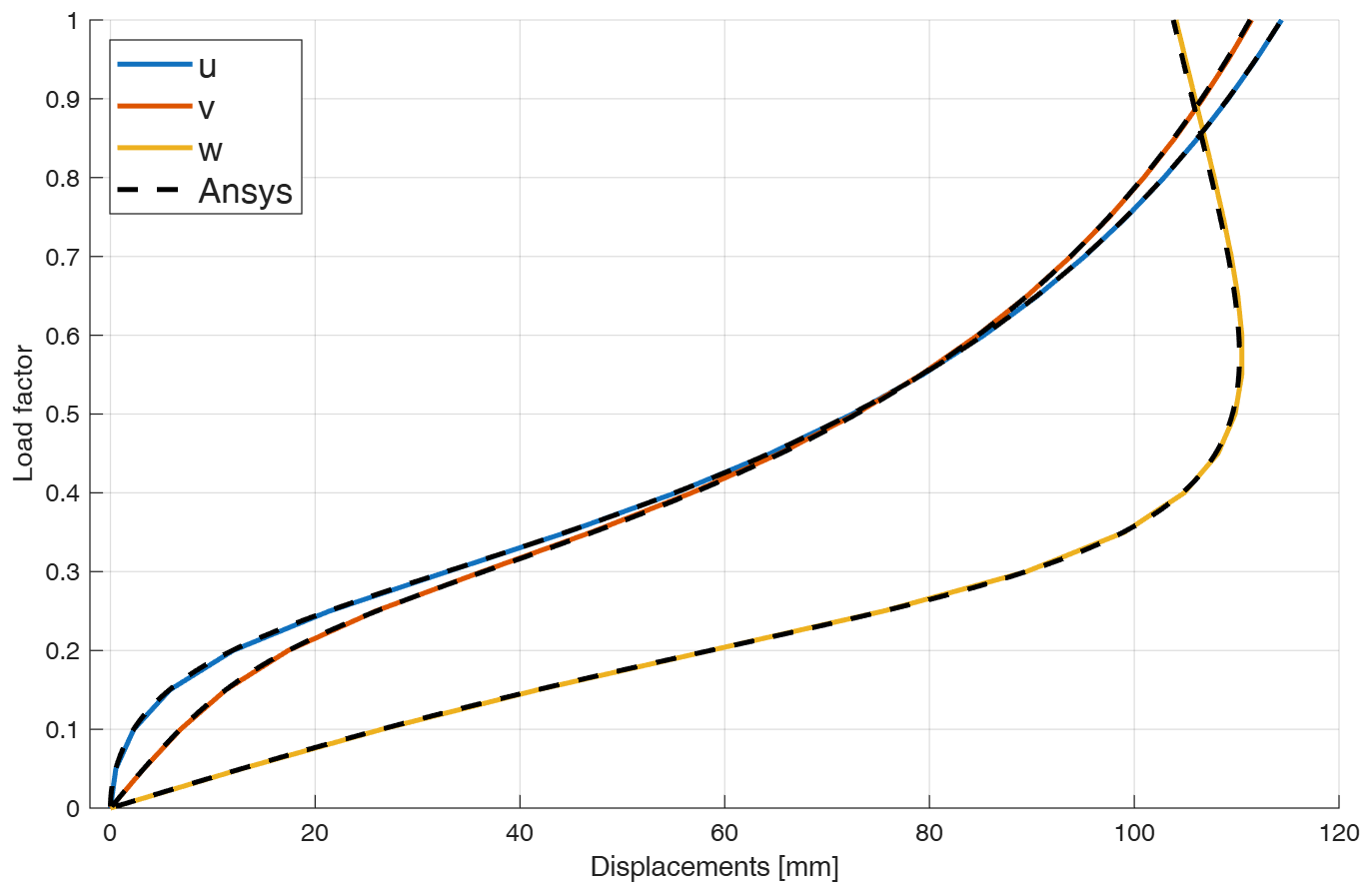
**Figure 2.** Load factor versus displacements [mm] for HEX20; dashed curves show the corresponding ANSYS results.

The HEX20 MATLAB results agree very closely with the corresponding ANSYS model. Likewise, the HEX8 MATLAB results in Section 26.1 agree with the corresponding ANSYS HEX8 results.

The noticeable difference between the HEX8 and HEX20 diagrams is therefore not evidence of an error in either MATLAB implementation. Each implementation reproduces the corresponding ANSYS element behaviour.

HEX8 mesh convergence

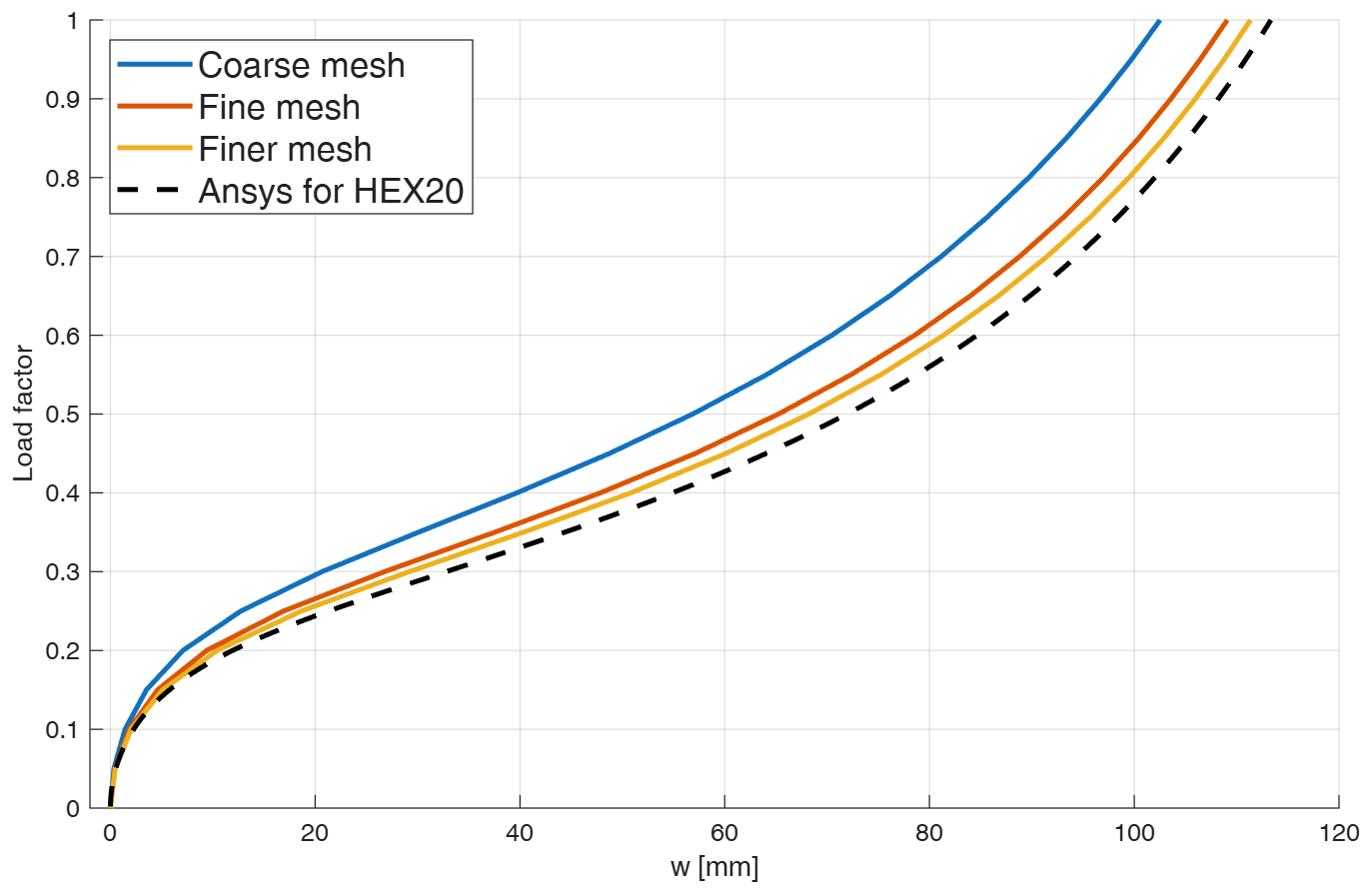
The convergence diagram for displacement $w$ compares three HEX8 meshes with the ANSYS HEX20 model described above:

Curve	Element	Mesh	Elements	Nodes	Equations
Coarse mesh	HEX8	50×6×4	1200	1785	5355
Fine mesh	HEX8	80×6×8	3840	5103	15309
Finer mesh	HEX8	120×6×6	4320	5929	17787
Ansys for HEX20	HEX20	30×4×2	240	1597	4791

**Figure 3.** HEX8 mesh convergence for displacement w [mm], compared with ANSYS for HEX20.

As the HEX8 mesh is refined, its solution progressively approaches that obtained with the HEX20 element. The substantial differences observed for the coarse HEX8 mesh are therefore mainly associated with the lower-order approximation and mesh discretization.

The comparatively stiff response of the coarse HEX8 mesh is characteristic of shear locking, which may affect low-order fully integrated elements in bending-dominated problems. As the HEX8 mesh is refined, this artificial stiffness decreases and the solution progressively approaches that obtained with HEX20. The higher-order HEX20 element is considerably less sensitive to this effect.

Locking phenomena and possible remedies will be discussed separately in a future section.

Conclusions and stress plots

The convergence study shows that the HEX8 solution progressively approaches the HEX20 result as the mesh is refined. The HEX20 element therefore provides, for this bending-dominated problem, a comparable response with a substantially coarser mesh.

This conclusion is supported by the numerical convergence study and by the agreement of both MATLAB implementations with their corresponding ANSYS element models.

The remarks in Section 26.1 concerning stress measures and the representation of stresses on the deformed configuration apply unchanged to HEX20. The transformation between second Piola–Kirchhoff and Cauchy stresses is discussed in Chapter 14.